
From 2,000+ Strategies to One Rebust System
A Data-Driven Journey into Trading System Design - Second Overview of A Quantitative Study of 30,000 Strategy Variations
1. Meta Description
This post presents a data-driven approach to trading system design, informed by the analysis of over 2,000 retail strategies using a proprietary research platform. We will explore the methodology behind the analysis, highlight consistent statistical behaviors across instruments and timeframes, and demonstrate how these insights can be translated into a robust, rule-based trading system suitable for automation.
2. Introduction
If you have traded for a while, most likely you have had a chance to wonder if some of the conditions you have been using actually help or break your system. In my posts, I will continue testing different combinations of technical indicator-based triggers to find out which combinations work best, which indicator should be excluded from the system, and how we can optimize the returns.
Let’s dive into the second post of historically profitable short term swing system analysis.
3. Methodology
3.1. Entry Triggers
3.1.1. Trigger: EMA[C, 3] > EMA[C, 6]
In this post, I will try to optimize the return even more by adjusting the triggers from the beginning. I’ve tested the following indicators on the chart, and they seem to highlight the conditions I would assume leading to a profitable system. Let’s see what we are going to work with:
Entry triggers:
- EMA[C, 3] > EMA[C, 6]:
- C < VWAP.14
- MACD[C, 6.12.7] > MACD[C.1, 6.12.7]
- EMA[(((V – V.1) * (C – C.1)) / (ATR[TR,1] * EMA[V, 4]), 5] > EMA[(((V.1 – V.2) * (C.1 – C.2)) / (ATR[TR,1.1] * EMA[V, 4.1]), 5]
- 1 < L.2
- C > C.1
- C > C.2
One of the most responsive signals in my system is a short-term exponential moving average (EMA) crossover: when the 3-day EMA crosses above the 6-day EMA. This trigger is designed to fire as soon as a potential short-term trend begins – perfect for traders looking for quick entries during early momentum phases.
Based on previous tests, the average holding period for the profitable system trades is around 6 to 10 days, making it ideal for short swing trades. With that timeframe in mind, I’ve adjusted the rest of the strategy components to better align with this rhythm.
Let’s see how this performs on a real chart.
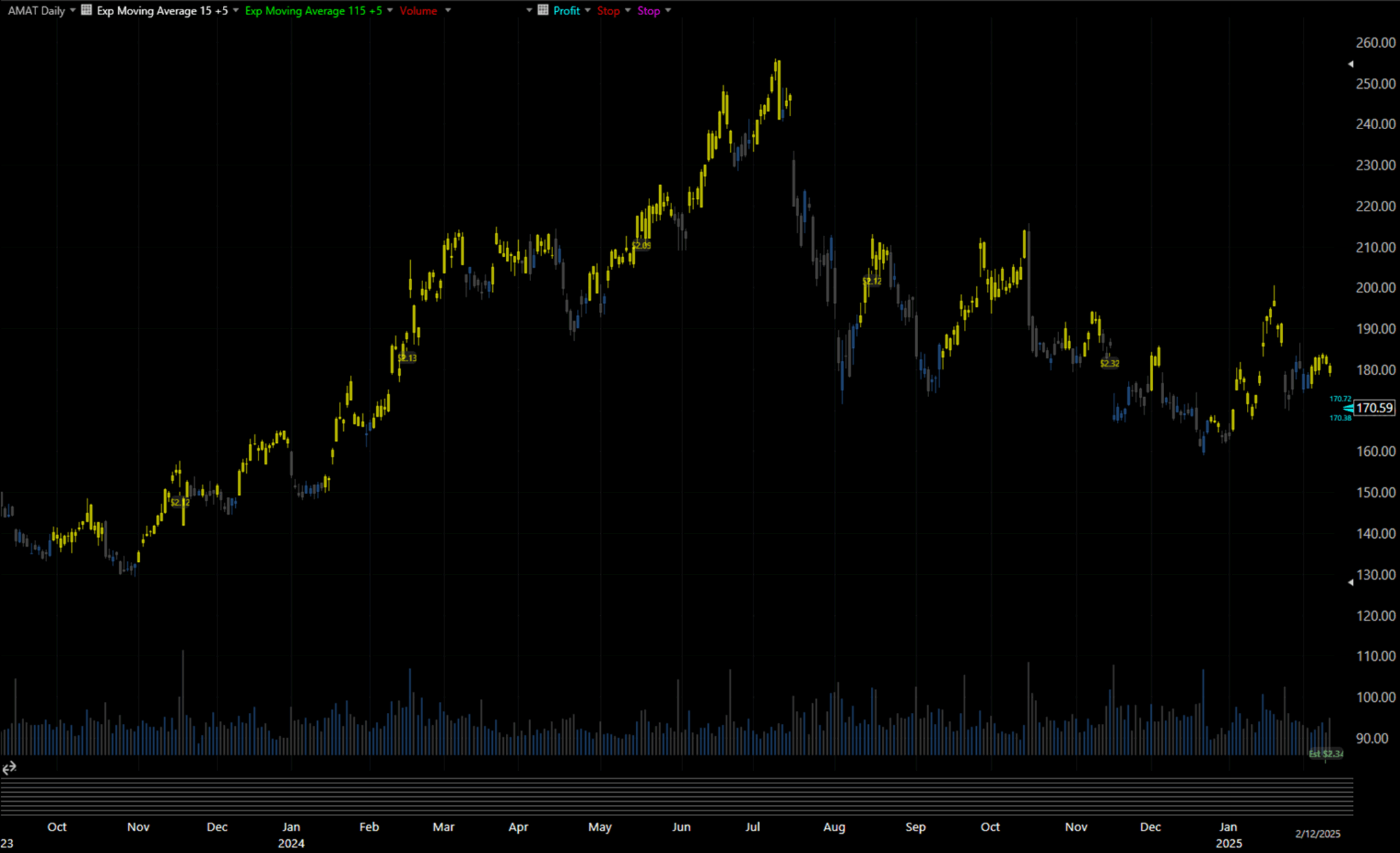
Figure 3.1.a – AMAT, September 2023 – February 2025
The chart above shows Applied Materials (AMAT) over a 17-month period. You’ll notice the yellow highlights marking where the 3-day Exponential Moving Average is above the 6-day Exponential Moving Average. As expected, there’s a fair amount of signal noise – short EMAs are extremely sensitive – but despite that, the trigger effectively identifies many of the early phases in strong uptrends.
These are the kinds of windows swing traders aim for: short bursts of momentum that can offer high reward within a short holding period.
3.1.2. Trigger: C < VWAP.14
This next trigger taps into a subtle yet powerful market condition: price falling below the 14-day Volume Weighted Average Price (VWAP). In plain terms, it flags moments when price dips aren’t being supported by volume – a key sign that a pullback may be nearing its exhaustion point.
Why is this useful?
In many cases, volume trailing behind price action suggests the market is losing conviction in the current move. So when the closing price is below a 14-day VWAP level, we’re often looking at the tail end of a downward move – a signal that a reversal or bounce may be close.
Let’s see it in action.
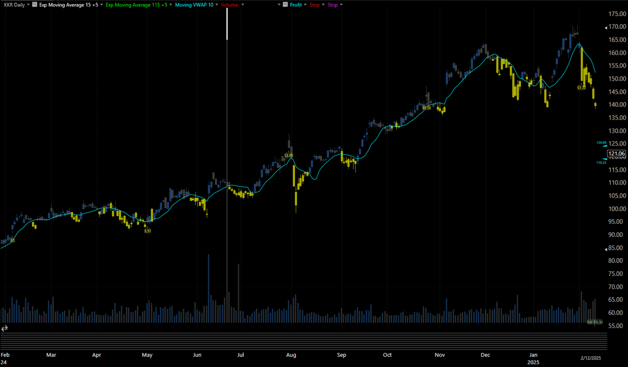
Figure 3.1.b – KKR, February 2024 – February 2025
The chart above shows how this trigger behaves across a year of trading KKR. The yellow highlights represent days where the closing price fell below the 14-day VWAP. You’ll notice it tends to cluster near short-term troughs – sometimes in strong downtrends, other times just before a bounce.
Yes, it’s noisy. But that’s by design. This trigger isn’t meant to be used in isolation. Instead, it specializes in catching moments of volume-price divergence – something that works best when cross-referenced with other indicators. As mentioned earlier, each part of the system is built to do one thing well. This one excels at flagging potential exhaustion during pullbacks, especially when a trend may be ready to resume.
3.1.3. Trigger: MACD[C, 6.12.7] > MACD[C.1, 6.12.7]
While some triggers aim to catch reversals or short bursts, others shine in trend-following. That’s exactly where this one fits in.
This trigger checks whether the MACD histogram (based on 6,12, and 7-day moving averages) is increasing compared to the previous day. In essence, it fires when the MACD is turning upward, signaling positive momentum building in the short-to-mid term. Depending on your overall system configuration, it can serve as either an entry trigger or a confirmation signal for ongoing trades.
Let’s take a look at how this plays out visually.
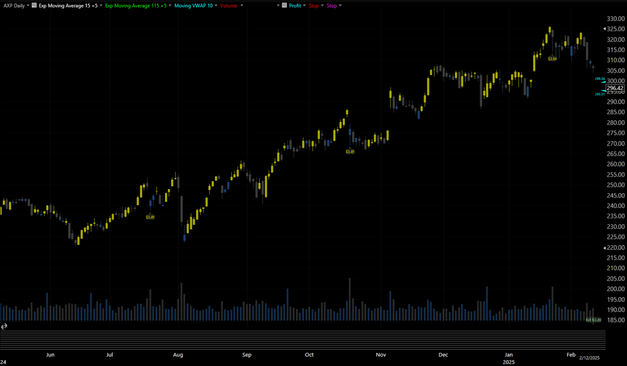
Figure 3.1.c – AXP, May 2024 – February 2025
In this American Express (AXP) chart, we see the MACD direction trigger doing exactly what it’s meant to do: activating early in the move and continuing throughout the price rally. The yellow highlights show how it tracked the upward push from start to peak, effectively aligning with the entire bullish leg.
This trigger works best in environments where momentum matters more than precision. It won’t catch every bottom, but it will often stay engaged through sustained climbs, keeping you in the trade as long as conditions remain favorable.
It’s especially valuable when used in combination with other filters, such as EMA crossovers or volume-based retracement checks, which help identify when the trend is starting and when it’s likely to end.
3.1.4. Trigger: EMA[(((V - V.1) * (C – C.1)) / (ATR[TR,1] * EMA[V, 4]), 5] > EMA[(((V.1 - V.2) * (C.1 – C.2)) / (ATR[TR,1.1] * EMA[V, 4.1]), 5]
This trigger is built for precision entries during potential reversals – but only when accompanied by a surge in volume. It’s a custom calculation designed to detect explosive shifts in behavior by comparing recent price/volume movement against previous momentum.
Put simply, this compares today’s price/volume shift normalized by volatility to that of the previous day. When the current impulse is greater, and backed by volume, it signals a strong potential turning point.
Let’s look at a recent example.
Figure 3.1.d – WMT, October 2024 – June 2025
At first glance, this chart may appear chaotic. Its purpose is to act as the final timing confirmation: when the setup is ready and other filters are aligned, this trigger tells you “Now.”
In the Walmart (WMT) chart above, we can see how this trigger doesn’t fire on every candle, but when it does, it tends to appear at key inflection points, especially those followed by meaningful continuation. It excels at highlighting high-momentum shifts that are backed by real participation.
Think of this one as the cherry on top – too reactive to rely on alone, but extremely valuable when other indicators agree. It ensures you’re not just seeing a price wiggle, but a momentum-backed event that’s worth your attention.
3.1.5. Triggers: L.1 C.1 and C > C.2
This next set of conditions may look deceptively simple – and that’s the point.
We’re breaking down a previously successful trigger into its individual components to analyze their standalone value. The logic here is:
- 1 < L.2: Yesterday’s low was lower than the day before.
- C > C.1: Today’s close is higher than yesterday’s close.
- C > C.2: And it’s also higher than the close from two days ago.
This combination essentially checks for a minor shakeout followed by bullish confirmation. The lower low indicates some intraday weakness or stop-run behavior, while the higher closes point toward buying pressure reclaiming control.
No flashy math here – just raw price action logic.
While this set doesn’t require a dedicated chart on its own, it represents an important stage of system optimization: deconstructing complex triggers to determine which parts truly carry predictive value. Sometimes, trimming the fat leads to a more agile, faster-reacting signal.
3.3. Entry Triggers
3.3.1. Structuring Risk and Capturing Opportunity
Even the best entry signals can fail without a solid exit strategy. That’s why this system’s exit logic is built to strike a balance between protecting capital and giving trades room to breathe.
Below is a breakdown of the current exit framework, including default parameters from previous iterations and some evolving logic based on early testing.
3.3.2. Profit Target
Formula:
Profit = C + (ATR[TR, 13] * 4)
This target sets the exit price at a level that is equal to four times the 13-day ATR added to the current closing price. It’s a relatively conservative yet opportunistic profit-taking mechanism. While not especially tight, this level is typically reached when the system’s indicators correctly anticipate a strong price move.
Think of it as a reward buffer – not overly aggressive, but definitely ambitious enough to capture the bulk of a short-term swing.
3.3.3. Stop Loss
Formula:
Stop = RANGE[L.L, 3] – ATR[TR, 13]
The stop loss follows the same logic used in earlier system versions: the lowest low of the past three days minus the 13-day ATR. This gives the trade some breathing room while still reacting to meaningful downside movement.
However, I’m considering revisiting this logic. In current testing, the 3-day low range has occasionally proven too disconnected from active price structure, especially in fast-moving or volatile environments. A wider or more adaptive structure may yield better results.
3.3.4. Trailing Stop
Formula:
If L > L.4 → Exit at RANGE[L.L, 6.1] – ATR[TR, 12.1]
This version introduces a refined trailing stop rule.
Instead of applying the ATR additively, we now subtract the ATR from the 6-day low range, both measured with a 1-day offset. This updated condition aims to better match rolling volatility behavior, locking in profits only after confirming a pivot or local top, while still allowing flexibility during the trend.
This logic ensures the trade is only exited after a lower-low sequence is broken, using a more dynamic floor rather than an arbitrary price level.
Now, let’s dive into the results.
4. Backtest Results: Digging into High-Return Configurations
To begin analyzing the backtest output, I sorted the results by return per trade, focusing only on configurations with sufficient sample size. I skipped low-sample outliers and narrowed in on the most promising candidates – specifically systems#36, #38, #43, and #46 or 2012221, 2112221, 2102221 and 2002221 respectively – each of which stood out for their performance.
Row # | Trades | Binary | Total Return (%) | Return per Trade (%) | Batting Average (%) | Avg Holding Time |
34 | 13 | 1121012 | 5.03 | 0.3873 | 38.46 | 12.1 days |
35 | 39 | 1112102 | 14.69 | 0.3767 | 41.03 | 19.8 days |
36 | 447 | 2012221 | 162.59 | 0.3637 | 41.7 | 19.4 days |
37 | 9 | 1011122 | 3.26 | 0.3626 | 33.33 | 17.0 days |
38 | 436 | 2112221 | 157.92 | 0.3622 | 41.38 | 19.3 days |
39 | 43 | 2220211 | 15.56 | 0.3619 | 39.53 | 18.2 days |
40 | 38 | 0212022 | 13.33 | 0.3508 | 50 | 21.8 days |
41 | 38 | 1212022 | 13.33 | 0.3508 | 50 | 21.8 days |
42 | 33 | 1112112 | 11.31 | 0.3426 | 39.39 | 19.8 days |
43 | 547 | 2102221 | 182.9 | 0.3344 | 40.11 | 18.8 days |
44 | 103 | 2021011 | 34.43 | 0.3342 | 38.83 | 17.9 days |
45 | 50 | 2222021 | 16.5 | 0.3301 | 42 | 19.8 days |
46 | 588 | 2002221 | 193.23 | 0.3286 | 40.2 | 18.9 days |
47 | 84 | 0211212 | 26.85 | 0.3196 | 41.67 | 18.6 days |
48 | 85 | 2021210 | 26.97 | 0.3173 | 40 | 18.2 days |
Table 4.a – High-Return Systems from raw data of Blog 2 back testing results, rows 34 to 48.
The key insight that stands out across these high-performing systems is this: the first condition (leftmost digit) is consistently set to ‘2’, meaning it was false. The next two conditions vary, but what really matters is that the final three conditions are also all false (222). In other words, many of the most profitable systems share a pattern of excluding certain signals, allowing just a few core conditions to drive performance.
This pattern is especially prominent in system 2002221, which is listed on line #46. With the highest total return in this group, it deserves a closer look.
To better evaluate whether this system has real trading potential and consistent performance, we need to dig deeper—by reviewing its individual trade entries and exits and visualizing how it behaves over time. Let’s begin with that.
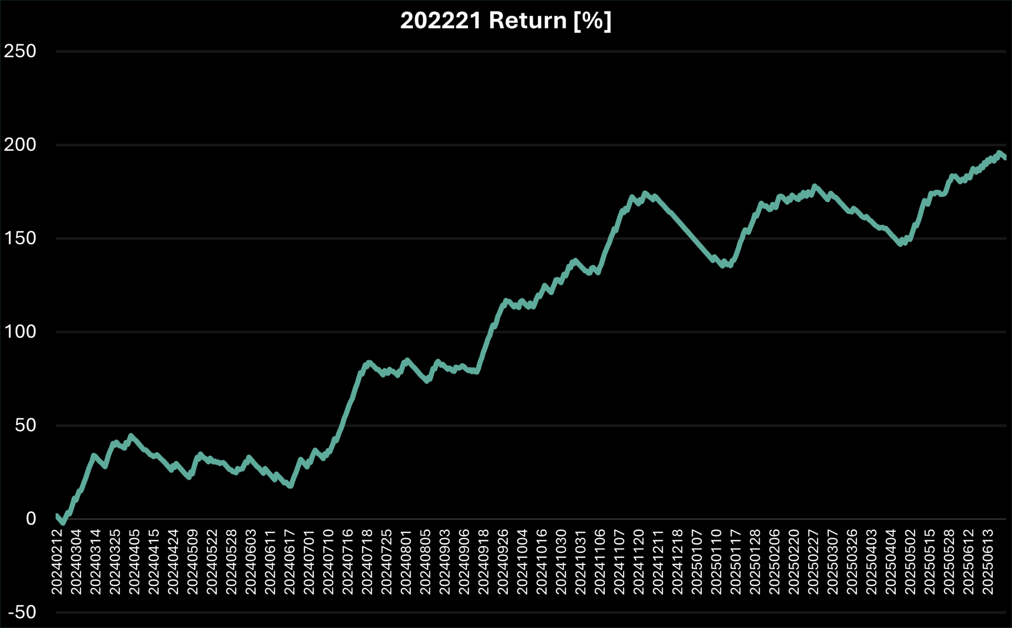
Figure 4.a – Return Over Time for System 2002221
The chart above shows the return progression for system 2002221, with each trade assuming a fixed 1% risk of total portfolio equity. The vertical axis reflects cumulative return in percentage terms, offering a clear visual of the system’s performance over time.
Even in this raw, unoptimized state, the equity curve demonstrates a consistently upward trajectory – a strong indication of structural reliability and potential robustness.
That said, there is still room for refinement. Adjustments to exit logic, or signal triggers could help reduce drawdowns and smooth out the equity curve further. However, caution is key: the system is already operating near the lower boundary of acceptable sample size. Over-filtering could remove too many trades, weakening statistical confidence and overall system viability.
The next step is to strike a careful balance—preserving the core behavior of the strategy while applying subtle optimizations that improve consistency without compromising depth or trade count.
4.3. Understanding what stands behind the system
Let’s now take a closer look at a sample trade chart generated by system 2002221. By reviewing these individual setups, we can gain a deeper understanding of why this specific combination of triggers works—and get a more intuitive sense of the market behavior it’s capturing. This visual layer helps bridge the gap between raw data and real-world context, showing exactly how and why the system engages with price action.
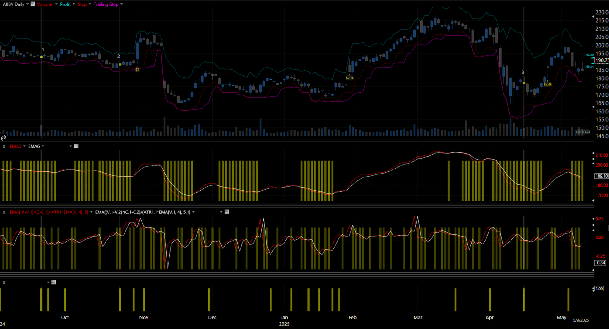
Figure 4.1.a – ABBV, September 2024 to May 2025
Let’s break down how the individual conditions within system 2002221 behaved in this trade example.
EMA3 < EMA6
This signal appears as the price begins to decline. It helps the system identify early-stage bottoms while avoiding overpriced entries during short-lived rallies. By waiting for this condition, the system positions itself to catch reversals at a discount.
Volume-Backed Pullback
The second trigger focuses on price declines accompanied by elevated volume. This often suggests that strong buying interest is starting to emerge—exactly the kind of pressure we want to see near turning points.
Price Action Trigger (Condensed Logic)
Rather than viewing the raw comparisons separately, I’ve grouped the following three into a single price action logic gate:
- 1 > L.2
- C < C.1
- C > C.2
Together, these paint a clear picture:
A day ago, the price showed relative strength (higher low). Today, that strength was broken with a drop in the closing price. Although the price dropped, the close is still higher than it was two days ago—suggesting that sellers may be losing control, and buyers are quietly stepping back in.
This sequence highlights controlled weakness followed by emerging support, a valuable structure in swing trading setups. It’s subtle, but when paired with the other conditions, it becomes a high-conviction entry.
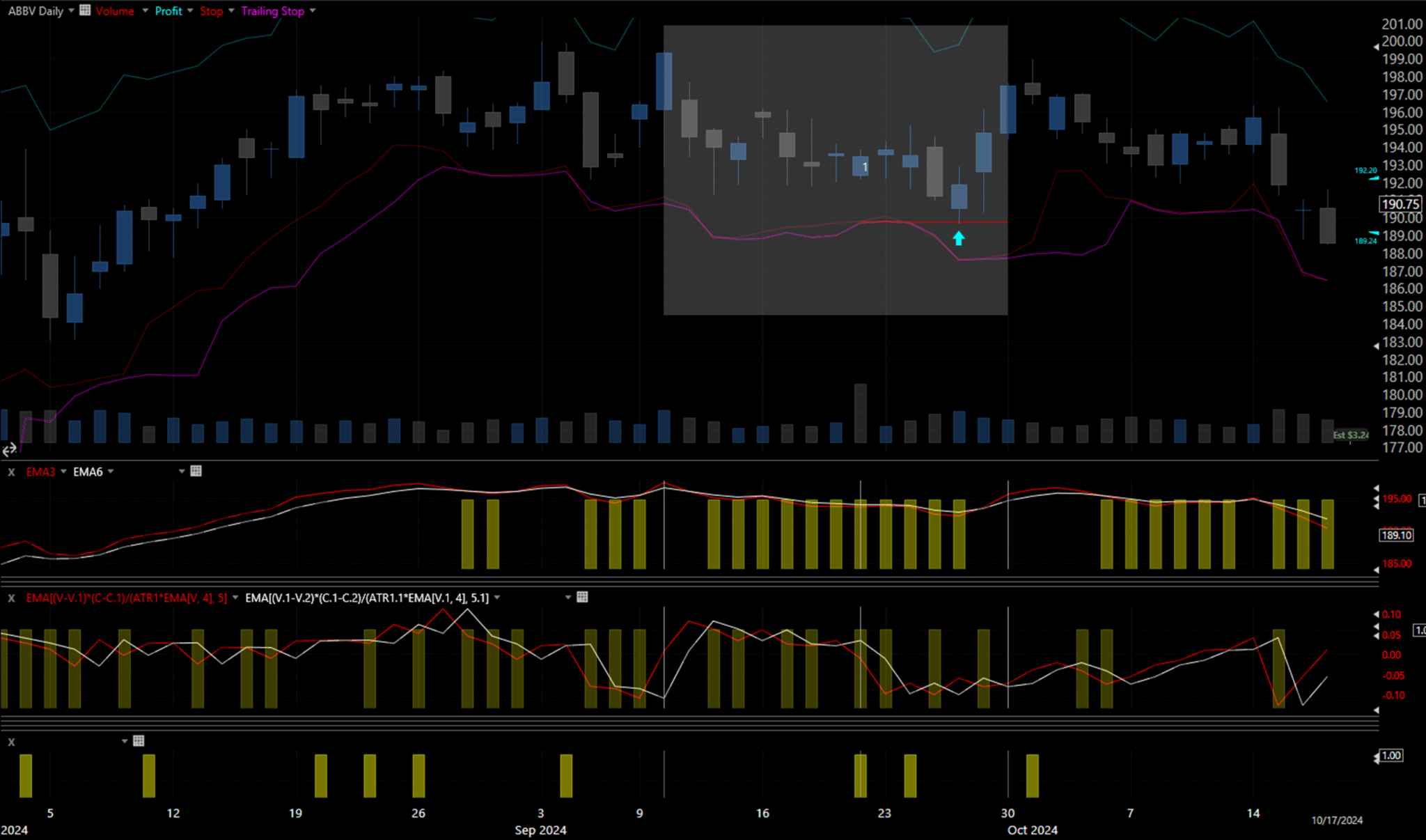
Figure 4.1.b – ABBV, August to October 2024
In this example, ABBV had just completed its first significant pullback following a strong three-month uptrend. Toward the end of the retracement, a notable setup occurred: the trading day opened with a gap down (where the digit “1” is marked), but most of the losses were recovered by the close. However, the closing price remained lower than the previous day’s, and the volume spiked significantly—triggering the system’s second condition related to volume-backed weakness.
The final signal in this setup came from a price action trigger that barely met the system’s threshold. The closing price hovered right between the two prior days’ ranges—an edge-case that could easily have failed to activate the signal had the price been just a few cents higher or lower. But of course, it’s easy to call it marginal with the benefit of hindsight.
What followed was a frustrating but instructive moment: within a week, the price dipped just far enough to hit the stop-loss target, only to reverse sharply and rally back up. Even a 15-pip adjustment would have kept the trade alive.
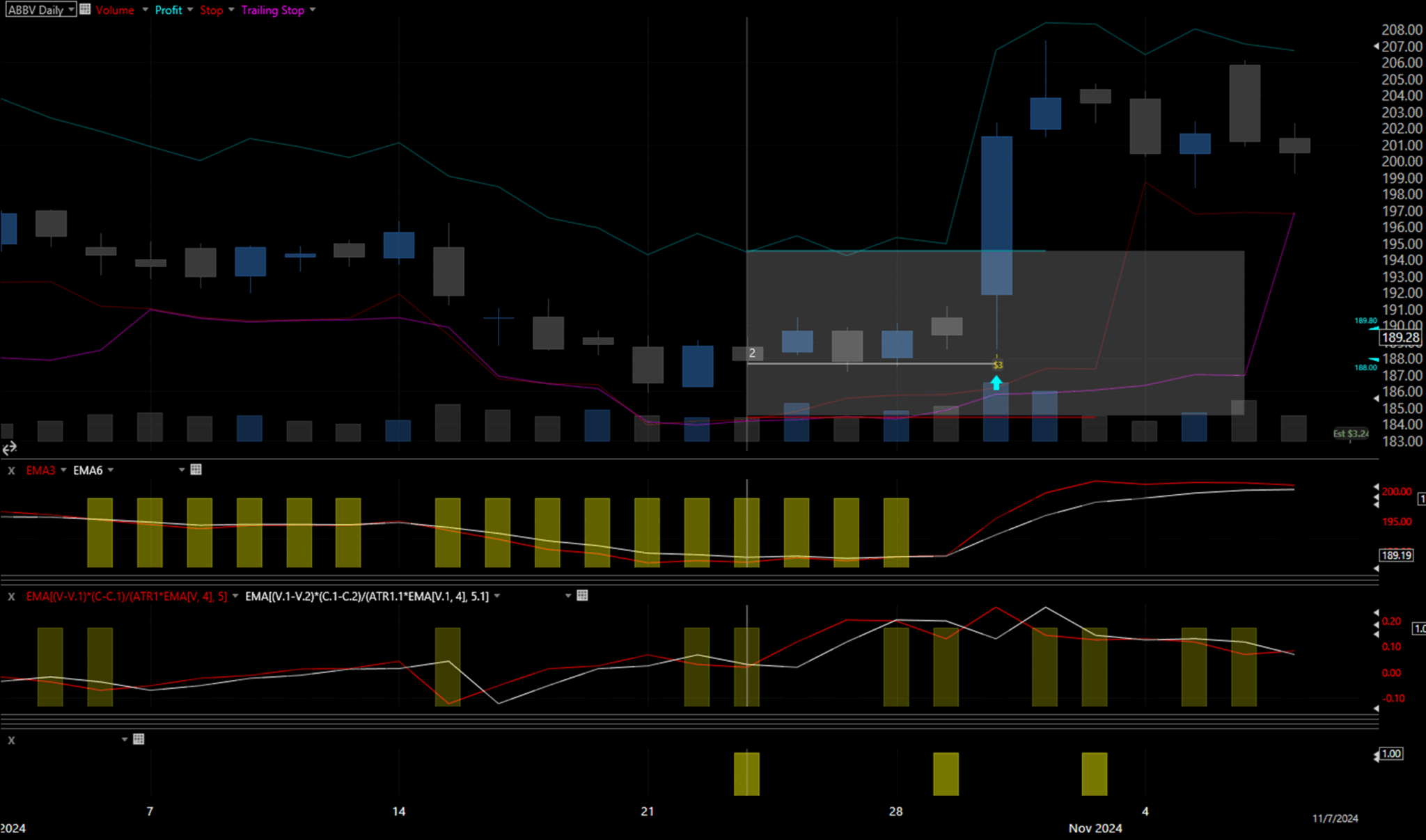
Figure 4.1.c – ABBV, October to November 2024
In this example, we see a familiar pattern playing out—another significant pullback following a prolonged move upward. The volume-based trigger activated during the continuation of a short-term downtrend, as captured by the declining 5-day EMA.
What makes this setup more favorable is how cleanly the combined price action trigger aligned. Two days earlier, the price featured a small-bodied candle partially engulfed by the next day’s strong close, then the price accumulated near a two-day high, supported by average volume. This suggested stabilization after the pullback and a controlled return of buying interest—an ideal environment for a swing entry.
The system entered the trade late in the week and closed the position early the following week, locking in a solid 2.5:1 reward-to-risk ratio.
This trade underscores the importance of alignment between all signals—particularly price structure and volume context. When these elements sync, the system shows its strength in capturing clean, high-probability opportunities with favorable risk profiles.
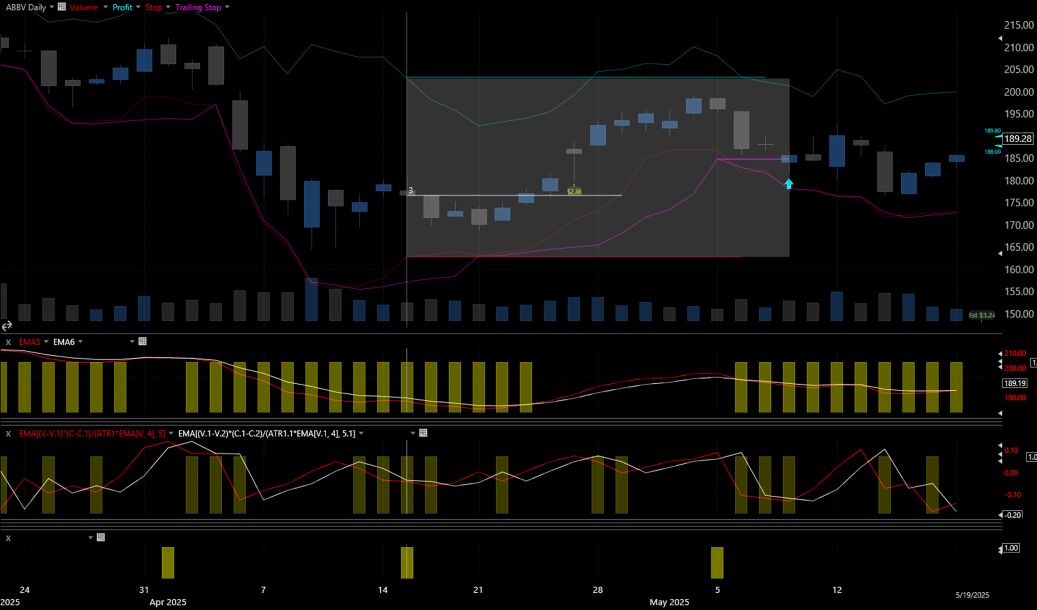
Figure 4.1.d – ABBV, Mid March to May 2025
Once again, a familiar setup emerges. After an extended period of downward pressure, price action begins to stabilize and show early signs of recovery—though overall sentiment remains cautiously bearish.
On the entry day, the combined trigger successfully identifies a micro pullback, allowing the system to enter at a moment when short-term weakness is starting to fade and momentum is beginning to shift upward.
The pullback continued slightly into the week, but was soon followed by a sharp 8-bar surge to the upside. Although the price didn’t quite reach the preset profit target, the system’s trailing stop activated at the right time, securing a return that equaled roughly 60% of the initial risk before the market began to pull back.
This trade clearly demonstrates the importance of a dynamic exit strategy. Even when the target isn’t fully met, the trailing stop adapts to real-time price action, protecting gains and reducing the risk of giving back profits on sudden reversals.
5. Adjusting the System Entry Triggeres
After reviewing multiple trade examples across various charts, one consistent failure pattern stood out: trades that lost money often had an entry-day low higher than the prior day’s low. This subtle but recurring detail suggested that entries taken without a proper intraday shakeout might be more vulnerable to reversal.
To test this theory, I introduced an additional filter that require the entry-day low to be less than the previous day’s low.
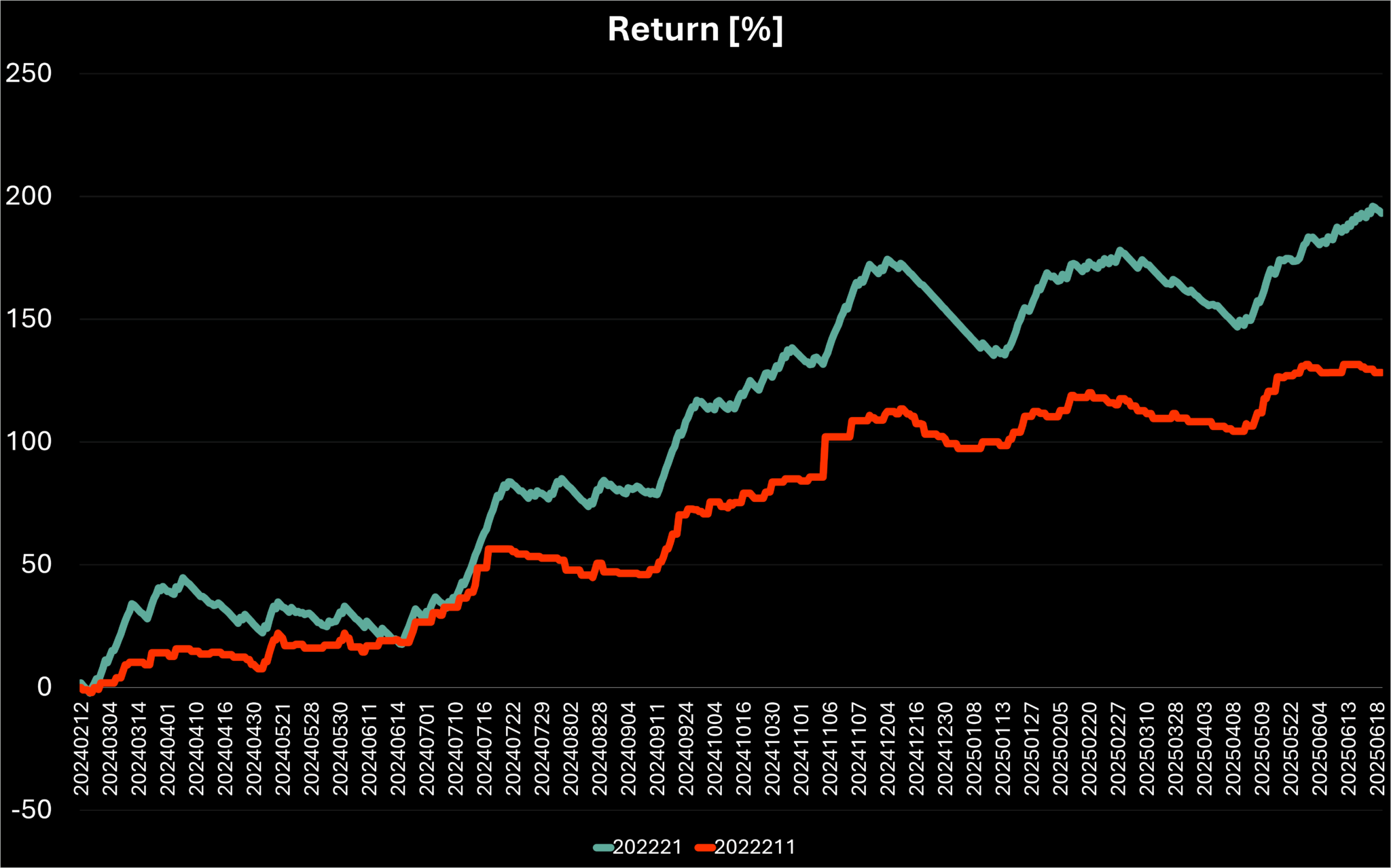
Figure 5.a – Return Over Time: Comparison Between Systems 2002221 and 2022211
The impact of this filter was significant:
📉 50% of trades were filtered out
📊 Total return dropped only 15%
📈 Return per trade increased by 68%
✅ Batting average improved by 15%
Visually, the equity curve (orange line) for system 2022211 is noticeably smoother and more consistent, showing fewer drawdowns and a much steadier climb. While some peak return was sacrificed, the trade-off appears highly favorable, transforming the system into one with stronger statistical confidence and improved reliability.
This result highlights the value of refining entry precision over simply chasing higher frequency. It suggests that even small structural adjustments—especially those grounded in price action context—can significantly improve a system’s stability without undermining its profitability.
5.3. Refining the Momentum-Volume Trigger
Next, let’s take a closer look at the following trigger:
EMA[((V – V.1) * (C – C.1)) / (ATR[TR, 1] * EMA[V, 4]), 5] < EMA[((V.1 – V.2) * (C.1 – C.2)) / (ATR[TR, 1.1] * EMA[V, 4.1]), 5]
This condition was originally designed to detect momentum shifts backed by volume, using a volatility-adjusted formula that compares recent price/volume acceleration against the previous day. To preserve the original structure of the trigger, I focused only on adjusting the volume EMA ranges (i.e., EMA[V, x]), keeping the rest of the logic intact.
Table 5.1.a – System Results by Volume EMA Range Adjustment. Performance metrics across different volume EMA lengths (adjusted symmetrically on both sides of the trigger)
This is a strong example of micro-adjustment in system tuning. Although the changes in volume EMA are relatively minor, the results offer useful insight. We can see that the shorter ranges (especially EMA[V, 3]) offer slightly better returns and a modest improvement in batting average—without introducing any instability or major shift in system behavior.
From a practical standpoint, it would not make sense to extend the volume range too far for a short-term swing system. The influence of volume on short-term moves is most effectively captured over smaller windows, and expanding that range tends to dilute its predictive power.
While the improvement from the 4-day EMA to the 3-day EMA is modest, it’s statistically consistent and directionally favorable. And since the optimization process is already in motion, I’ll incorporate this micro-adjustment into the system—giving it the benefit of the doubt, and prioritizing clarity and responsiveness in volume analysis.
5.3.1. Evaluating the Inner EMA Range of the Volume-Momentum Trigger
Next, I examined the effect of adjusting the inner EMA range used in the volume-momentum function—specifically the moving average applied to the function itself on both sides of the equation:
EMA Smoothing Period (X) | Total Return (%) | Return per Trade (%) | Batting Average (%) |
3 | 133.88 | 0.4448 | 42.19 |
5 (original) | 169.97 | 0.5762 | 46.78 |
10 | 169.73 | 0.5423 | 45.37 |
15 | 141.22 | 0.4399 | 42.37 |
23 | 141.58 | 0.4239 | 41.62 |
Figure 5.a – Performance metrics based on different EMA lengths applied to the trigger function
Among all the tested variations, the original 5-day EMA remains the most effective. It strikes the best balance across total return, return per trade, and batting average. Shorter or longer EMA windows either weakened the signal’s responsiveness or smoothed it to the point of reduced impact.
Given these results, there’s no compelling reason to alter the original configuration. I’ll leave this condition as-is and move on to the final trigger in the system to evaluate whether it offers any room for meaningful improvement.
5.4. Adjusting the Relative EMA Ranges
To preserve the structural relationship between the short- and long-term EMAs, I began by adjusting both sides of the trigger proportionally:
EMA[C, X] < EMA[C, Y],
with X and Y scaled together by the same percentage
This ensures that the relative responsiveness of each average remains consistent across all tests, allowing us to isolate the effect of speed (range) without distorting the logic of the trigger.
EMA Range (Short, Long) | Total Return (%) | Return per Trade (%) | Batting Average (%) |
1, 3 | 185.43 | 0.3242 | 38.99 |
3, 6 (original) | 169.97 | 0.5762 | 46.78 |
5, 10 | 160.42 | 0.4583 | 44 |
7, 14 | 170.27 | 0.4446 | 44.13 |
9, 18 | 176.37 | 0.4169 | 43.74 |
Figure 5.2.a – Performance by Proportionally Adjusted EMA Ranges. System results for different proportional EMA pairings in the trigger
What stands out in this table is a familiar trade-off:
Shorter EMA ranges (e.g., 1/3) lead to a higher number of trades due to increased sensitivity, which in turn boosts total return.
However, this comes at a cost—return per trade and batting average decline, reflecting the trigger’s tendency to fire in more volatile or uncertain conditions.
While the increase in total return is notable, it’s driven by frequency rather than precision. The drop in quality metrics suggests a less efficient signal, which may not justify the added exposure and execution cost in a real-world scenario.
In contrast, the original setting (3 and 6-day EMA’s) maintains the best overall balance—strong return per trade, solid hit rate, and a reasonable trade frequency—making it a strong candidate to keep as the default for this trigger.
5.4.1. Evaluating Trade Efficiency: Return per Trade vs. Batting Average
To get a clearer view of the system’s behavior, I visualized the two most important performance metrics—Return per Trade (RpT) and Batting Average (B.A.)—across the range of proportional EMA settings:
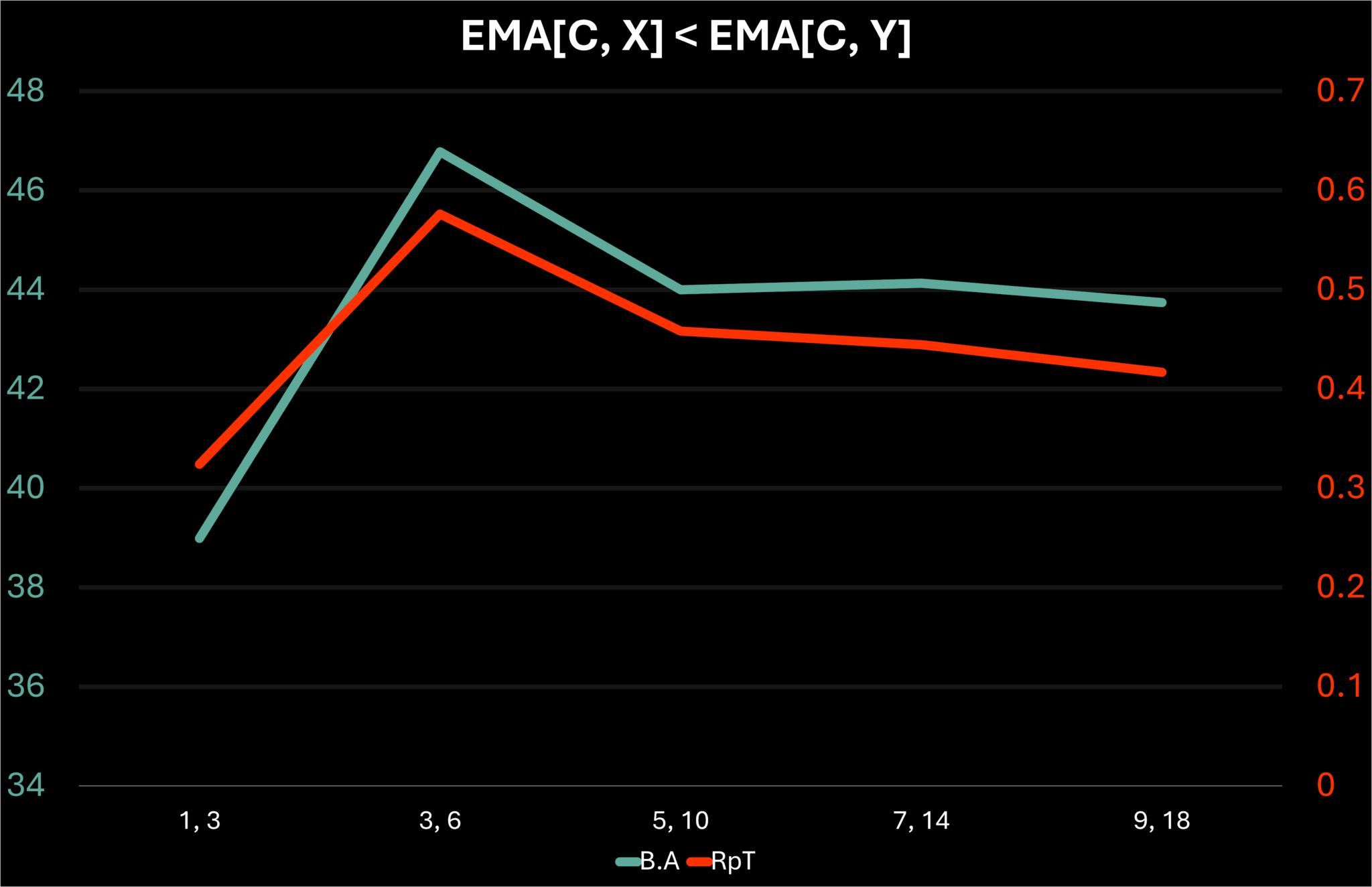
Figure 5.2.a – RpT and B.A. by EMA Range Pair (Symmetrical Scaling). B.A and RpT comparison for different exponential moving average ranges changing the same percentage on both sides of the trigger EMA[C, X] < EMA[C, Y].
The chart above makes it clear: the 3 and 6-day EMA’s combination remains dominant across both performance metrics. On the left side of the plot, shorter ranges (1 and 3-day EMA’s) increase trade frequency but reduce quality—leading to a steep drop in both RpT and B.A. This is consistent with earlier findings: faster signals tend to trigger more frequently but often under less favorable conditions.
On the right side of the chart, longer EMA combinations also underperform. But the cause here isn’t just lag; it’s that the rest of the system’s components—already tuned around a short-term swing structure—no longer sync well with these slower trigger values. It’s not that 3 and 6 are optimal in isolation—it’s that they cohere well with the surrounding logic.
Conclusion
The sharp decline in both metrics on either side of the 3/6 pairing suggests that this range provides the best balance of timing, precision, and compatibility within the broader system.
That said, optimization is never fully complete. Even though the main adjustment phase is wrapping up, there’s still one more logical direction to explore—asymmetric EMA combinations. While left-side values below 3 leave little room without micro-tuning, we can still test alternative structures by changing the relationship between short and long EMA’s. This might reveal new system behaviors worth considering.
Let’s move forward with that.
5.4.2. Asymmetric Adjustment: Tuning the Right-Side EMA Only
To further refine the system, I tested the impact of asymmetric EMA ranges, this time adjusting only the right side of the condition:
EMA[C, 3] < EMA[C, Y]
This approach keeps the faster EMA range as 3-day fixed, while systematically increasing the smoothing of the slower EMA. The idea is to see if a more pronounced divergence between the short- and long-term trend could yield improved system behavior.
EMA Range (Short, Long) | Total Return (%) | Return per Trade (%) | Batting Average (%) |
3, 4 | 136.75 | 0.4798 | 42.46 |
3, 6 (original) | 169.97 | 0.5762 | 46.78 |
3, 9 | 148.05 | 0.4656 | 43.71 |
3, 12 | 146.77 | 0.4381 | 43.28 |
3, 16 | 157.68 | 0.4467 | 43.63 |
3, 19 | 159.31 | 0.4413 | 43.49 |
3,21 | 158.02 | 0.4259 | 42.86 |
Figure 5.2.b – System results with fixed short EMA (3) and varying long range EMA
The pattern here is consistent with earlier findings:
Reducing the long EMA to 4-day range results in a significant drop in both RpT and B.A., likely due to increased signal noise and premature entries.
Increasing the long EMA beyond the original 6-day range initially leads to a modest decline in performance, followed by a brief recovery around the 16-day and 19-day regions.
However, the longer the range becomes, the less aligned it is with the system’s short-term swing trading goals, and the performance metrics begin to decline again.
While the 16 and 19-day ranges configurations produced slightly higher total returns than the original, these gains came with lower efficiency per trade and only marginal improvement in trade quality—likely not enough to justify the added lag and deviation from the system’s intended timeframe.
Final Takeaway for Trigger Adjustment
This final round of testing confirms what we’ve observed throughout: the original 3 and 6-day EMA combination remains the most balanced configuration across key performance metrics and aligns best with the system’s structural goals.
With this, we conclude the main phase of trigger optimization. The next step is to analyze and refine the system’s exit logic—evaluating how different closing strategies affect overall performance. This will complete the structural foundation of the system before moving on to robustness testing, walk-forward validation, or live model integration.
6. Adjusting the System Exit Triggers
6.3. Tuning the Profit Target
6.3.1. Adjusting the ATR Multiplier
We now turn to optimizing the exit logic, starting with the profit target. While entries and exits have the same influence on shaping equity curve behavior, the profit target itself tends to have less sensitivity compared to trailing stops or stop-loss logic—making it a logical first candidate for review.
The profit target is calculated as:
Exit Price = C + (ATR[TR, 13] × X)
Where X is the multiplier being tested. Below is a comparison of system performance across different X values:
ATR Multiplier (X) | Total Return (%) | Return per Trade (%) | Batting Average (%) |
1 | 64.54 | 0.2043 | 72.47 |
2 | 98.41 | 0.3269 | 56.81 |
3 | 137.62 | 0.4649 | 48.99 |
4 (Original) | 169.97 | 0.5762 | 46.78 |
5 | 149.54 | 0.5341 | 42.86 |
6 | 149.83 | 0.5448 | 41.45 |
7 | 140.43 | 0.5163 | 40.07 |
Figure 6.1.a – System results with different ATR multipliers used for profit targets
As expected, lower ATR multipliers (e.g. 1–3) lead to higher batting averages, since targets are more easily reached. However, this comes at a cost: return per trade and total return both fall sharply, as gains are capped too early, leaving significant profit on the table during strong moves.
While some traders may prefer this approach to achieve smoother equity curves or higher win rates, the drop in overall efficiency is too steep to justify the trade-off in this case.
On the other side of the spectrum, raising the ATR multiplier beyond 4 yields diminishing returns. Although RpT remains respectable, the win rate declines and total return begins to fade—likely due to more frequent reversals before reaching increasingly distant targets.
Conclusion
The original ATR multiplier of 4 remains the best-balanced setting—offering a solid mix of return potential, trade quality, and system consistency. I’ll keep this parameter unchanged and proceed to the next (and more sensitive) component: the stop-loss logic.
6.3.2. Adjusting the ATR Calculation Window
Next, I explored how changes to the ATR calculation range affect the system’s performance. This is the length of the window used to measure volatility in the following formula:
Profit Target = C + (ATR[TR, X] × 4)
The multiplier remains fixed at 4, while the value of X (the ATR range) is adjusted to see how short- and long-term volatility measures influence trade outcomes.
ATR Range (X) | Total Return (%) | Return per Trade (%) | Batting Average (%) |
4 | 148.31 | 0.5062 | 46.08 |
7 | 158.95 | 0.5481 | 45.86 |
10 | 155.47 | 0.5417 | 45.99 |
13 (original) | 169.97 | 0.5762 | 46.78 |
16 | 153.27 | 0.534 | 45.64 |
19 | 149.35 | 0.5222 | 45.8 |
Figure 6.1.b – Performance with different ATR ranges used in the profit target formula
Once again, the original setting (13-day ATR) delivers the best overall result across key metrics. Shorter ATR windows, 4 to 10-day range, result in slightly less consistent profit targets due to increased responsiveness to short-term volatility spikes. This can lead to overly conservative exits during trending conditions.
Conversely, longer ATR windows (16 to 19-day range) tend to smooth out short-term noise but may lag behind active price dynamics, occasionally setting overly ambitious targets during volatile periods. This makes them less suited for a system aiming to capture swing moves within 1–2 weeks.
From visual chart reviews, the original target consistently produced profit targets that align with typical price expansion following a valid signal—often hit within ~7–10 trading days after entry. While some trades exceed the target significantly and others fall just short, the average outcome suggests that this range is well-calibrated to the system’s time horizon.
Conclusion
The current ATR setting of 13 continues to make the most sense—both statistically and visually. Further improvements may be possible, but likely only through multi-variable optimization or real-time adaptive targeting, which would require a Phase 2 analysis after validating the system in live or forward-testing conditions.
For now, I’ll retain the existing value and move forward to the stop-loss logic, which has a much more direct effect on capital protection and trade outcomes.
6.4. Evaluating the Stop Target: ATR Multiplier Adjustment
Let’s now focus on the stop target, a parameter with greater influence on overall system performance than the profit target—especially when it comes to drawdown control. While the trailing stop ends up closing most trades, the initial stop is what sets the system’s maximum risk tolerance per trade, making it a key component of capital protection.
As with the profit target, I tested various ATR multipliers using the following stop-loss formula:
Stop = Lowest Low over X bars – (X * ATR[13])
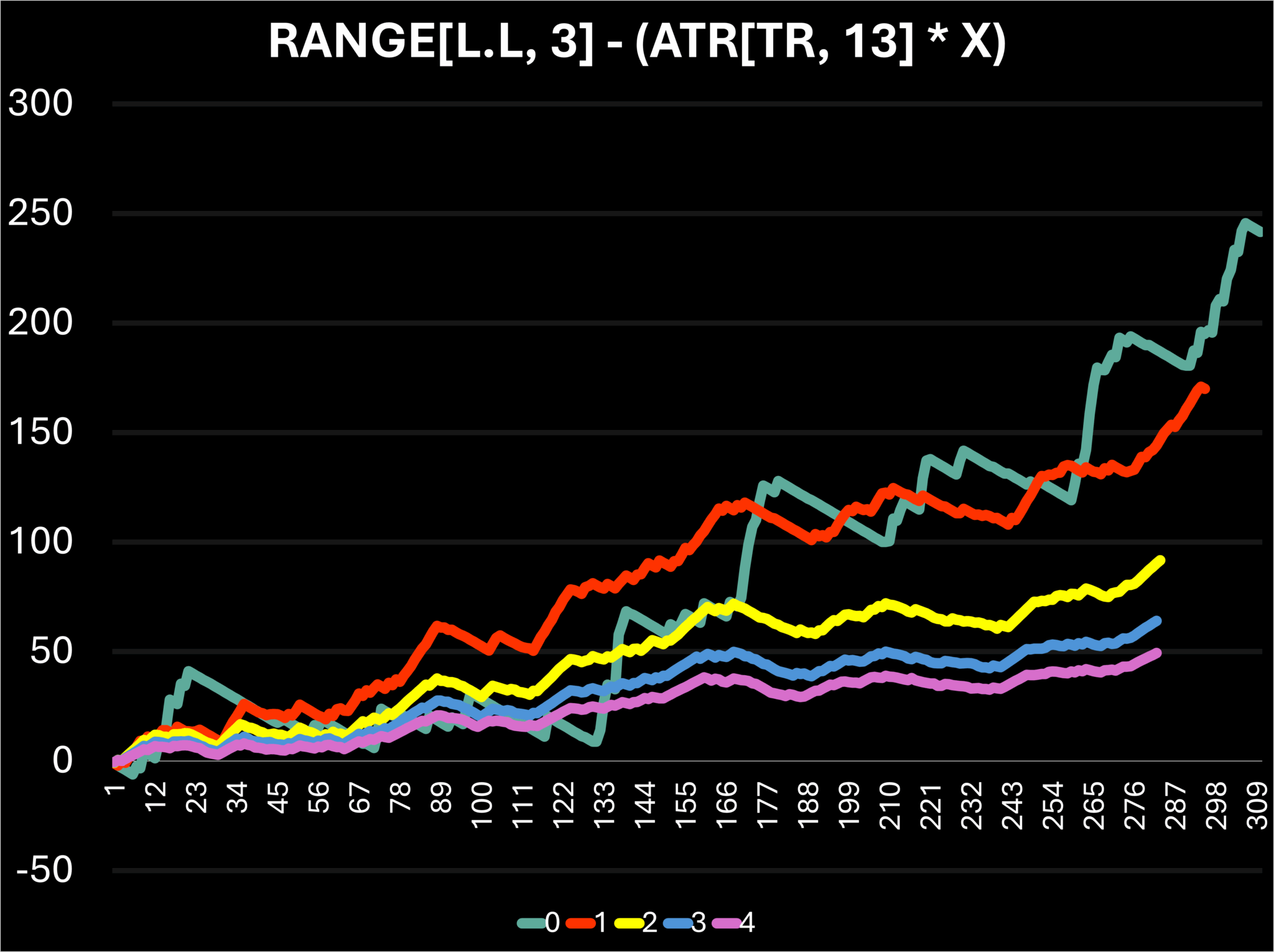
Figure 6.2.a – System Return Using Different ATR Multipliers for the Stop Target
In this case, I chose to display the results as a chart rather than a table. That’s because the chart helps highlight a misleading assumption: at first glance, the zero-multiplier line (X = 0) appears to produce the highest total return. However, that comes at a steep cost—the batting average drops to around 23%, which is a 50% decline from the baseline.
This instability is clearly visible in the chart. Without an ATR component, the system becomes overly reactive, leading to wild equity curve swings and inconsistent performance. The system may catch a few big trades, but it’s also far more exposed to noise and false breakouts.
As we increase the ATR multiplier, the stop becomes looser, giving trades more breathing room. While this makes the system more stable, both return per trade and total return begin to decline. In other words, more conservative stops reduce trade exits from noise, but at the cost of efficiency.
Conclusion
Among all the options tested, the original setting (ATR multiplier = 1) once again provides the best balance between risk control, return consistency, and overall system quality. It avoids the volatility of an overly tight stop while preserving enough structure to keep the system disciplined.
6.4.1. Testing the Lower Low Range
The final component of the stop target formula to evaluate is the Lower Low range, which determines how many bars the system looks back to define the recent lowest price. The stop formula being tested is:
Stop = Lowest Low over X bars − ATR[13]
Below are the results of testing different values for X:
|
Lower Low Range (X) |
Total Return (%) |
Return per Trade (%) |
Batting Average (%) |
|
1 |
153.62 |
0.5316 |
42.91 |
|
2 |
153.62 |
0.5316 |
42.91 |
|
3 (original) |
169.97 |
0.5762 |
46.78 |
|
4 |
149.67 |
0.5233 |
46.15 |
|
5 |
153.34 |
0.538 |
47.02 |
|
6 |
147.45 |
0.5174 |
47.02 |
|
7 |
145.97 |
0.5122 |
47.02 |
|
8 |
138.09 |
0.4845 |
47.02 |
Figure 6.2.a – System Performance by Lower Low Range (X)
The results here are very straightforward: the original 3-day lookback for the lower low yields the highest return, highest efficiency per trade, and the most balanced win rate.
Shorter ranges (1–2 days) offer lower batting averages accompanied by slightly lower efficiency and return, while longer ranges (4–8 days) gradually erode both return per trade and total return—even as the batting average slightly improves. This suggests the system becomes too tolerant, allowing trades to float further into loss territory before cutting.
Once again, this reinforces how well the original configuration is aligned across multiple components. There’s no advantage in changing this range, and doing so would only weaken the system’s overall responsiveness and capital protection.
Conclusion
With the lower low range confirmed at 3, the initial stop structure is now fully optimized. What’s becoming increasingly clear is that while the stop target plays an important role, most of the system’s exit performance is being driven by the trailing stop.
6.5. Trailing Stop Trigger: Testing the Lower Low Comparison Range
The trailing stop in this system is controlled by two separate formulas:
Trigger condition – This determines when to update the trailing stop:
L > L.4
Meaning the trailing stop is only recalculated if today’s low is higher than the low from 4 days ago.
Trailing stop value – Once the condition is met, the stop is set using:
Trailing Stop = RANGE[L.L, 6.1] − ATR[TR, 12.1]
In this section, we’ll focus on the first part—the comparison range used in the update condition (i.e., how many days back to compare today’s low with).
Lower Low Comparison Range (X) | Total Return (%) | Return per Trade (%) | Batting Average (%) |
2 | 142 | 0.5053 | 44.84 |
3 | 156.31 | 0.539 | 45.86 |
4 (original) | 169.97 | 0.5762 | 46.78 |
5 | 152.65 | 0.5264 | 45.86 |
6 | 154.41 | 0.5343 | 45.33 |
7 | 148.62 | 0.509 | 46.23 |
Figure 6.3.a – System Performance by Lower Low Lookback in Trailing Stop Trigger
Once again, the original setting (L > L.4) proves to be the most effective. It delivers the highest return, highest return per trade, and strongest win rate across all tested variations.
This trigger acts as a gate for updating the trailing stop. If it’s too short (e.g., 2 or 3 days), the system becomes overly sensitive, leading to frequent updates and potential overreactions. On the other hand, if it’s too long (5 to 7 days), the updates come too late—often after momentum has faded—reducing effectiveness and return quality.
Conclusion
This is the first system I’ve deeply analyzed where nearly every original parameter consistently outperforms all tested alternatives. It appears to be extremely well-calibrated right out of the gate, which gives me high confidence in its real-world potential.
If even the value-setting formula for the trailing stop turns out to be optimal without modification, that would be a rare outcome – and one worth observing closely as the system evolves in live conditions.
6.5.1. Trailing Stop Value: Tuning the Lookback Offsets
Now that the update trigger logic has been confirmed, it’s time to focus on the value assigned when the trailing stop is updated.
The formula currently in use is:
Trailing Stop = RANGE[L.L, 6.1] − ATR[TR, 12.1]
In this section, I’ll test variations of the offset applied to both components—the lower low range and the ATR—simultaneously. The goal is to evaluate whether giving the stop more room or tightening it yields better performance.
Offset (X) | Total Return (%) | Return per Trade (%) | Batting Average (%) |
0 | 155.37 | 0.5376 | 47.06 |
1 (original) | 169.97 | 0.5762 | 46.78 |
2 | 148.83 | 0.5259 | 45.23 |
3 | 142.11 | 0.5057 | 44.13 |
Figure 6.3.b – System Performance by Lookback Offset in Trailing Stop Calculation
As the offset increases, giving the trailing stop more historical data to average over (i.e., making it more conservative), we see a gradual drop in all the parameters. This is expected—wider trailing stops offer more breathing room, but at the cost of letting more losses run and missing early exit signals.
Interestingly, tightening the trailing stop by removing the offset (using recent day values) leads to the highest win rate 47.06%, slightly above the original value of 46.78%. However, this comes with a modest decrease in both RpT and total return.
The original offset of 1-day still provides the best overall balance, producing the highest return and maintaining solid trade efficiency. It seems to give the system just enough flexibility to let trades run, without being overly exposed to short-term volatility.
Conclusion
This test further reinforces the notion that the current system is remarkably well-calibrated. While minor improvements in win rate can be achieved by tightening the trailing stop, it comes at the cost of return potential. Once again, the original configuration (1-day offset) emerges as the optimal setting.
In the next step, I’ll isolate and examine the Lower Low component of the trailing stop value formula to determine if its specific range can be fine-tuned independently for further enhancement.
6.5.2. Trailing Stop Value: Lower Low Range Adjustment
With the trailing stop update logic and offset optimized, the next step is to analyze the lookback period used in the Lower Low component of the trailing stop formula:
Trailing Stop = RANGE[L.L, X.1] − ATR[TR, 12.1]
Here, I tested different values for X, the number of bars over which the lowest low is calculated.
Lower Low Range (X) | Total Return (%) | Return per Trade (%) | Batting Average (%) |
3 | 131.39 | 0.4439 | 46.28 |
4 | 152.46 | 0.5257 | 47.59 |
5 | 155.03 | 0.5383 | 46.88 |
6 (original) | 169.97 | 0.5762 | 46.78 |
7 | 153.34 | 0.5418 | 45.58 |
8 | 149.28 | 0.5294 | 45.04 |
9 | 148.22 | 0.5275 | 44.48 |
Figure 6.3.c – System Performance by Lower Low Lookback (X) in Trailing Stop Calculation
While slightly higher batting averages were achieved by tightening the range as for 4 and 5-days, they came at the cost of lower overall return and efficiency. Similarly, increasing the lookback window gradually decreased all performance metrics, signaling less responsiveness and potentially slower stop adjustments.
Once again, the original setting (6-day lower-low lookback) proves to be the most balanced, delivering the best combination of return, RpT, and consistency. The smaller improvements in win rate from other configurations aren’t compelling enough to justify sacrificing return potential.
Conclusion
The system continues to demonstrate strong alignment between components. While small tweaks offer marginal changes, they do not justify moving away from the original value. This reinforces confidence in the system’s internal harmony.
We’re now down to the final parameter—the ATR range used in the trailing stop value calculation. While expectations are low at this point for a meaningful improvement, it’s worth validating.
6.5.3. Final Trailing Stop Adjustment: ATR Lookback
The last parameter to evaluate is the lookback range used in the ATR component of the trailing stop calculation. This value affects how responsive the stop level is to recent price action.
ATR Range (X) | Total Return (%) | Return per Trade (%) | Batting Average (%) |
8 | 154.32 | 0.5358 | 45.83 |
9 | 154.57 | 0.5386 | 45.99 |
10 | 153.98 | 0.5365 | 45.99 |
11 | 156.9 | 0.5467 | 45.99 |
12 (original) | 169.97 | 0.5762 | 46.78 |
13 | 155.89 | 0.5432 | 45.99 |
14 | 155.57 | 0.5421 | 45.99 |
15 | 155.2 | 0.5408 | 45.99 |
Figure 6.3.d – System Performance by ATR Lookback (X) in Trailing Stop Calculation
Summary
This final test confirms the pattern: the original 12-day setting consistently delivers the best results, both in total return and return per trade. Remarkably, this system is the first in my entire research that performed so well from the outset it needed only one meaningful adjustment.
The likely explanation? A rare and powerful synergy between its technical triggers—where even minor tweaks throw the system off balance. This reinforces a key insight: some systems within the 2,180 tested combinations are already finely tuned by design. You don’t always need to over-optimize; sometimes, the right combination just works.
What’s Next?
I’ll be adding this configuration to my live watchlist to track its real-time behavior. If it continues to deliver under real market conditions, this could become a serious candidate for active deployment in my own trading.
If you’re interested in exploring any of the rest 2,179 back tested combinations, you can find:
A full summary file of all results, with Individual trade files for each configuration and a more detailed breakdown of additional parameters that categorize each of these combinations.
⬇️ All of these are available for download below. Whether you’re looking for short-term setups, high batting averages, or robust long-term systems—there’s likely something here that fits your trading style. If you would like to see this and many other systems system combinations that may have even greater historical performance values from a list of 2,180 samples, that suit your style of trading, you can find all of the individual files for each combination and a summary list with all the system performances down below
— End of Part Two
⚠️ Disclaimer
The content provided in this post is for informational and educational purposes only. It represents my personal research, observations, and experimentation with trading systems, and is not intended as financial advice, investment advice, or a recommendation to buy or sell any securities or financial instruments.
Trading in the financial markets involves significant risk, and you should never invest money you cannot afford to lose. The systems discussed here were tested using historical data under specific assumptions, and past performance is not indicative of future results. Market conditions change, and no strategy can guarantee profits or prevent losses.
While I strive to be as transparent and data-driven as possible, all results, charts, and conclusions are presented as-is and may contain errors, omissions, or inaccuracies. Any decisions to trade based on this content are made entirely at your own risk. I disclaim all liability for any financial loss, damage, or consequences that may result from the use of the information provided here.
Please consult with a licensed financial advisor, legal professional, or risk specialist before engaging in any trading or investment activity.