
From 2,000+ Strategies to One Rebust System
A Data-Driven Journey into Trading System Design - First Overview of A Quantitative Study of 30,000 Strategy Variations
1. Meta Description
This post presents a data-driven approach to trading system design, informed by the analysis of over 2,000 retail strategies using a proprietary research platform. I explore the methodology behind the analysis, highlight consistent statistical behaviors across instruments and timeframes, and demonstrate how these insights can be translated into a robust, rule-based trading system suitable for automation.
2. Introduction
In this post, I’ll walk you through a data-driven approach I used to evaluate 2,180 systematically generated trading strategy variations, each tested across more than 200 U.S. equities over a two-year historical period. This large-scale effort was powered by a custom-built research and analytics platform, purpose-designed for rapid, high-volume backtesting and performance comparison.
Each strategy was derived from combinations of seven distinct technical triggers, tested across every possible logical configuration. For each condition, the system could require it to be true, explicitly false, or ignored altogether – allowing for a wide and nuanced variation in logic. (I’ll break down this rule-coding system in the next section.)
The primary objective wasn’t just to identify high-performing systems, but to isolate those that are robust, interpretable, and aligned with my own trading style. Throughout the process, I also refined parameters to improve clarity and reduce unnecessary complexity – without sacrificing performance. This marks the first step in transforming statistical insights into a practical, rule-based trading system, suitable for eventual automation.
3. Methodology
At the core of this study lies a structured combinatorial framework built around seven technical indicators, each of which can be configured in one of three states:
- 0 – The condition is ignored (not part of the logic)
- 1 – The condition must be true
- 2 – The condition must be false
This simple encoding creates a matrix of all possible logic combinations. Each unique permutation results in a 7-digit strategy identifier, representing a fully defined trading rule set. The system cycles through every valid configuration, resulting in thousands of distinct strategies – all tested under identical market conditions for comparative consistency.
Each strategy was backtested using two full years of historical data, beginning on March 31, 2023. The stock universe – consisting of over 200 U.S.-listed equities – was carefully curated based on criteria tailored to short-term swing trading. This included filters for liquidity, daily volume, volatility, market capitalization, and price behavior, ensuring that the strategies were tested on realistic and tradable instruments.
Many of the trigger conditions are built on established technical indicators such as:
- Exponential Moving Average (EMA)
- Moving Average Convergence Divergence (MACD)
- Average True Range (ATR)
- Volume-based momentum factors, and more.
These indicators were used to define entry conditions, exit points, profit targets, and stop-loss logic. Each strategy represents a unique synthesis of these elements, offering insights into both classic and unconventional trading behaviors.
A key feature integrated into nearly all systems was a trailing stop-loss mechanism. Prior testing has shown that this dynamic exit strategy can significantly improve risk-adjusted returns, particularly by locking in gains during trend reversals. While some strategies may show higher raw returns without it, I consider a well-designed trailing stop to be essential for capital protection and risk control – two principles at the heart of my systematic trading philosophy.
3.1 A Quick Note on Interpreting Indicators Systematically
If you’re accustomed to interpreting indicators visually on a chart, it’s important to recognize that their behavior can look very different in a fully systematic environment. Once human discretion is removed and rigid entry/exit logic is applied at scale, familiar technical patterns often behave in unfamiliar ways. What looks effective on a handful of charts may fail – or behave completely differently – when tested across hundreds of instruments and thousands of trades.
This is precisely why rigorous backtesting is essential. It reveals how indicators actually perform under consistent, rule-based application – rather than how they appear in hindsight.
To illustrate this point, let’s explore the foundational conditions used in this study.
3.1.1 Trigger: EMA[C, 27] > EMA[C, 17]
At first glance, this appears to be a classic trend-following signal, comparing two exponential moving averages. The rule tests whether the longer-term average is currently positioned above the shorter-term average. Traditionally, traders interpret this as a bearish signal, often associated with the onset of downtrends or the end of upward momentum. But when applied programmatically across a wide dataset, its behavior becomes more nuanced and context-dependent.
Here’s what the data reveals:
- In downtrending markets: This condition tends to trigger with a slight delay, and may continue holding true until a strong rally appears. It doesn’t reliably signal the start of a downtrend – but it often confirms it.
- In sideways or range-bound markets: The signal often lags behind price action, triggering after the dip has already begun. This reduces its usefulness as a proactive filter.
- In strong uptrends: Surprisingly, this condition can act as a bottom-finder, sometimes triggering just before short-term rebounds within a broader bullish move. This happens because pullbacks can briefly reverse the EMA positioning before a continuation rally resumes.
- In choppy or indecisive markets: The signal becomes noisy and unreliable, with frequent crossovers that fail to lead to consistent outcomes.
This variability is exactly what makes this rule valuable to test within a larger system. By embedding it into a matrix of complementary conditions, we can isolate when it adds value, and when it doesn’t.
Throughout the analysis, I’ll be exploring several key questions for this and every other entry condition:
- Does this rule improve results when set to True (EMA[27] > EMA[17])?
- Is its inverse (EMA[27] < EMA[17]) more effective?
- Or is the best-performing version the one that excludes this condition altogether?
By evaluating these outcomes across thousands of strategy combinations, I aim to turn intuition-driven chart patterns into data-backed decisions. This is where discretionary trading ideas begin to evolve into structured, testable hypotheses – forming the foundation for reliable, rule-based systems.
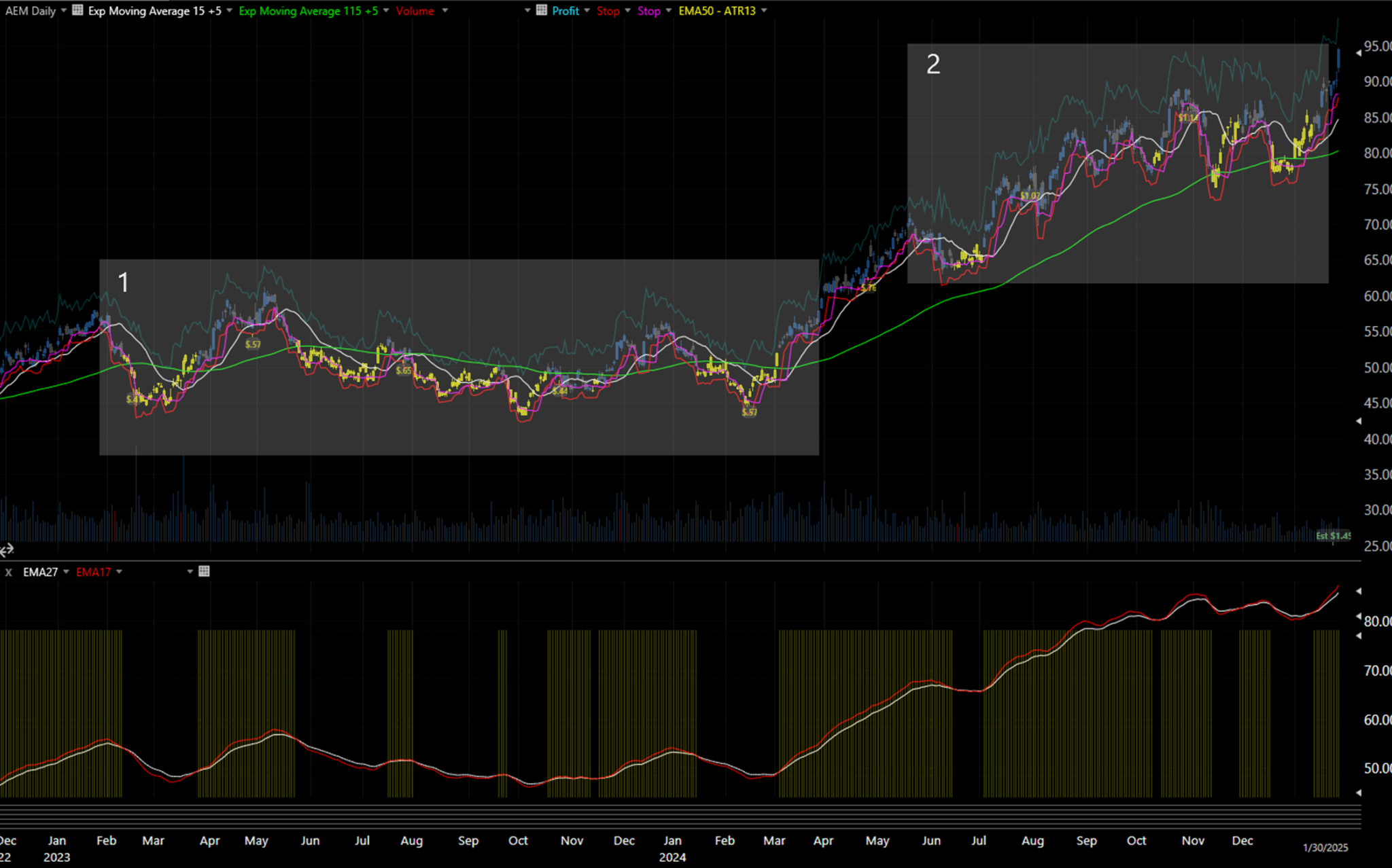
Figure 3.1.a — This chart illustrates the behavior of the condition EMA[C, 27] > EMA[C, 17] applied to Agnico Eagle Mines (AEM) over a two-year period.
Yellow candlesticks mark periods when the condition is true, while yellow markers beneath the chart offer a secondary visual reference for its activation. The white line represents the 27-day EMA, and the red line shows the 17-day EMA—making it easy to observe how their crossover dynamics evolve across different market phases.
Observe how the signal behaves across different market regimes:
- In choppy or range-bound conditions (Area 1), the trigger tends to flicker on and off, producing frequent and often unreliable signals. This instability reflects the lack of directional conviction and can undermine the effectiveness of the rule in volatile, non-trending environments.
- In sustained uptrends (Area 2), the condition occasionally aligns with short-term pullbacks, offering some potential for timing long entries. However, its precision remains limited—it does not consistently mark ideal entry points, but it can serve as a loose proxy for bullish continuation setups.
This visual highlights both the potential value and contextual limitations of using this rule as a long-side filter in systematic strategies. Like many trend-following indicators, its effectiveness depends heavily on the broader market structure—and must be evaluated in combination with complementary signals to avoid false confidence.
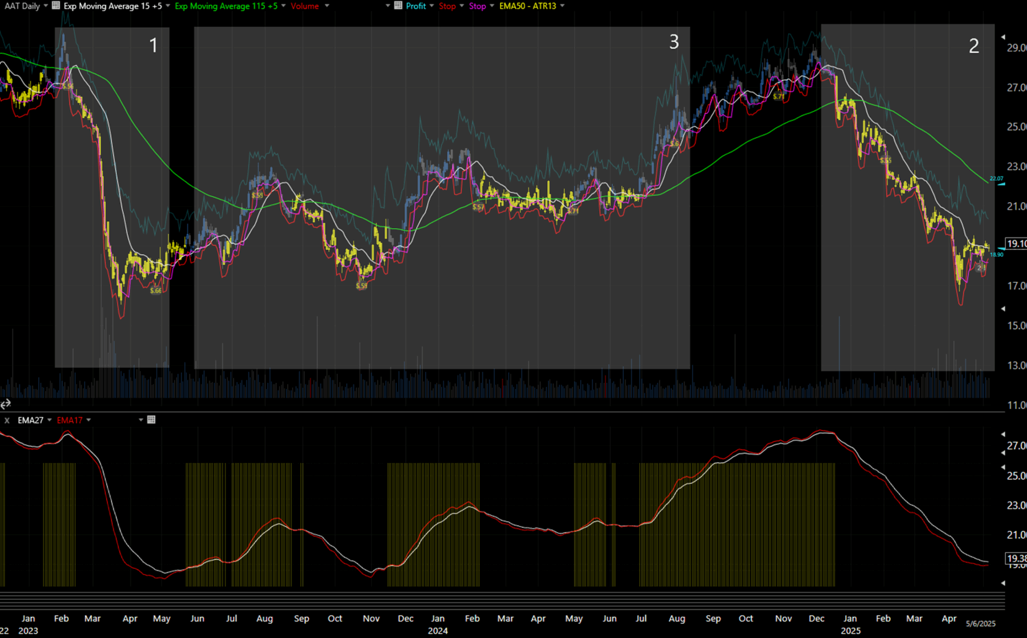
Figure 3.1.b — This chart demonstrates the behavior of the condition EMA[C, 27] > EMA[C, 17] applied to Caesars Entertainment Corp (CZR) over a two-year period.
As with previous examples, yellow candlesticks and yellow signal bars below the chart indicate when the condition is true. This visual offers additional context for how the trigger responds during trend reversals, consolidations, and volatile transitions—reinforcing its strengths and limitations across varying market conditions.Notice how the signal behaves across varying market environments:
- During extended downtrends (Areas 1 and 2), the condition tends to activate with a slight delay, aligning more with continued weakness than early reversals—making it more of a confirmation tool than a predictive one.
- In sideways or consolidating markets (Area 3), it produces intermittent signals, reflecting its heightened sensitivity in non-trending phases. This often introduces noise that can reduce its standalone reliability.
This figure reinforces what we saw in the earlier example: the effectiveness of this trigger is highly context-dependent. As such, it’s best suited for selective use within long-biased systems, particularly when paired with complementary filters that can help distinguish trend strength from indecision.
Figure 3.1.c — This chart illustrates the behavior of the condition EMA[C, 27] > EMA[C, 17] applied to Agnico Eagle Mines (AEM) over a two-year period.
The white line represents the 27-day EMA, and the red line shows the 17-day EMA—making it easy to observe how their crossover dynamics evolve across different market phases.
Observe how the signal behaves across different market regimes:
- In choppy or range-bound conditions (Area 1), the trigger tends to flicker on and off, producing frequent and often unreliable signals. This instability reflects the lack of directional conviction and can undermine the effectiveness of the rule in volatile, non-trending environments.
- In sustained uptrends (Area 2), the condition occasionally aligns with short-term pullbacks, offering some potential for timing long entries. However, its precision remains limited—it does not consistently mark ideal entry points, but it can serve as a loose proxy for bullish continuation setups.
This visual highlights both the potential value and contextual limitations of using this rule as a long-side filter in systematic strategies. Like many trend-following indicators, its effectiveness depends heavily on the broader market structure—and must be evaluated in combination with complementary signals to avoid false confidence.
3.1.2 Trigger: EMA[C, 115.5] - EMA[C, 15.5] < ATR[TR, 65.5] * 0.6
This condition functions as a long-term trend stability filter, intended to distinguish early-stage accumulation phases from deeper pullbacks or prolonged markdowns—while accounting for recent volatility.
It works by measuring the distance between a half-year exponential moving average (115.5 days) and a shorter, three-week EMA (15.5 days), and comparing that difference to 60% of the 65-day Average True Range (ATR). If the short-term EMA hasn’t significantly undercut the long-term EMA—relative to the stock’s typical volatility—the condition evaluates as true. This implies a potentially constructive setup where the price is not overly deteriorated.
Why the Unconventional Parameters?
The original intention behind this configuration was to approximate a weekly trend-following signal. The 5-day offset synchronizes daily data with Friday closes, which often serve as the anchor for weekly chart evaluations—especially when executing entries at the end of the trading week. That said, I may later test alternative configurations (e.g., a 1-day offset) and adjust the EMA/ATR lengths to better fit different entry styles.
Strategic Application
In my framework, this rule is used primarily as a background filter rather than a direct entry condition. Its role is to confirm a structurally healthy environment—typically a period of accumulation where price begins to compress and stabilize. This compression, reflected in a narrowing gap between the long- and short-term EMAs, may precede bullish expansion.
However, one major caveat is signal instability. When the condition frequently toggles between true and false—especially due to the 5-day offset—it becomes unreliable. This flip-flopping can occur in noisy or volatile environments, degrading the condition’s value. In such scenarios, I prefer to set this rule to return false, effectively filtering out setups where price action has decayed too far beneath the long-term average.
In summary, this condition helps screen for trend continuity and constructive basing behavior, reducing the likelihood of entering long trades in deteriorating market environments. When used appropriately, it can serve as a valuable structural safeguard that helps long-only systems avoid fading momentum.
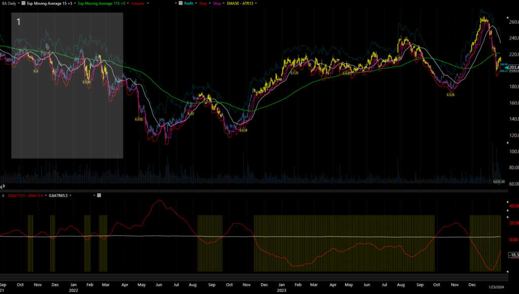
Figure 3.1.d — This chart demonstrates the condition EMA[C, 115.5] – EMA[C, 15.5] < ATR[TR, 65.5] * 0.6 as applied to Boeing (BA) between August 2021 and January 2024.
The bottom panel displays the difference between the long- and short-term EMAs (in red), plotted against 60% of the 65-day ATR (white line). Highlighted yellow zones represent periods where the condition evaluates to true.
Observe how the condition tends to activate during low-volatility, compression phases, particularly in early-stage accumulation zones. However, its reliability declines when volatility increases—causing the signal to flicker erratically or fire late during strong moves, especially during the first half of the chart (Area 1). This underscores the condition’s value as a broad-phase filter, rather than a timing signal—useful for excluding deteriorating setups in long-only strategies.
3.1.3 Trigger: MACD[C, 7.15.5] > MACD[C.1, 7.15.5]
This condition uses a short-term configuration of the Moving Average Convergence Divergence (MACD) to detect near-term shifts in momentum. Specifically, it compares the current day’s MACD value with the previous day’s reading. If today’s value is greater, the condition evaluates as true, suggesting that bullish momentum is strengthening. Conversely, if today’s MACD is lower, it returns false, signaling a possible loss of momentum or early reversal.
While subtle in construction, this condition introduces an important directional timing component to strategy design. It doesn’t just identify whether momentum exists—it helps determine whether that momentum is increasing or fading, which is critical when managing entries in fast-moving or breakout-prone environments.
Strategic Implications
If this trigger adds value to a system’s overall structure, it will most commonly do so when the condition is true—confirming that positive momentum is building, and supporting long entries.
That said, there are edge cases. In ultra-early entry strategies, for example, some profitable trades may actually begin when momentum is just about to shift—making a false condition potentially useful. These setups aim to anticipate rather than confirm price acceleration, so the strategic role of this trigger depends heavily on the system’s time horizon and risk posture.
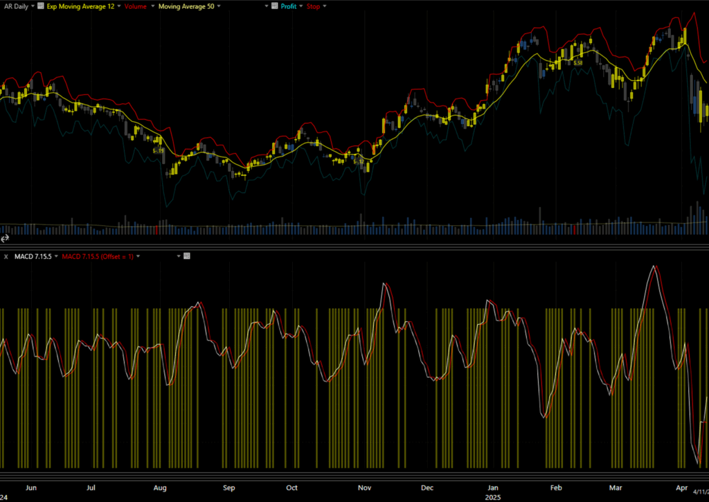
Figure 3.1.e — This chart illustrates the condition MACD[C, 7.15.5] > MACD[C.1, 7.15.5] applied to Antero Resources (AR) between June 2024 and April 2025.
The yellow bars in the lower panel represent periods when the condition evaluates to true—signaling that the current MACD value exceeds that of the previous day and indicating rising short-term momentum.
This condition performs particularly well in identifying early momentum shifts, often triggering ahead of brief uptrends or price recoveries. In contrast to broader trend indicators, this logic focuses on momentum inflection points, offering tactical advantages for traders seeking precise timing—especially in volatile or mean-reverting environments.
Note how the signal aligns with all price surges, during pullbacks, providing not just entry signals but also helping avoid overstaying positions during weak retracements.
Because of its sensitivity, this condition may be less effective on its own in choppy markets—where false positives can occur frequently—but when paired with broader trend filters, it adds a valuable layer of entry precision to systematic strategies.
3.1.4 Trigger: EMA[(V × (C − C.1)) / ATR[TR, 1], 5.1] > 0
This condition evaluates volume-weighted price momentum, normalized by short-term volatility. The formula multiplies the daily price change (C − C.1) by volume (V), then divides by the 1-day Average True Range (ATR[TR, 1]) to adjust for market noise. Finally, it applies a 5.1-period EMA to smooth the result—creating a dynamic momentum signal that responds to both price direction and volume intensity.
A value greater than zero indicates that price is rising on expanding volume, signaling strong, conviction-driven buying. A value less than zero reflects price change occurring on declining or weak volume, which can be a warning sign of momentum fading or even a precursor to reversal.
This condition is adaptable and particularly effective when paired with other signals. Its role varies depending on strategic context:
- Used as False: It may validate controlled pullbacks or soft corrections in a broader downtrend, where volume confirms the move’s integrity.
- Used as True: It helps confirm genuine upside thrusts—especially useful in differentiating between weak rallies and sustainable moves backed by volume.
By incorporating both price change magnitude and trading volume, this rule acts as a volatility-adjusted momentum filter, which enhances precision in environments where simple price-based signals might mislead.
Its responsiveness makes it especially useful in short-term systems aiming to fine-tune entries during breakouts, rebounds, or continuation setups—where volume confirmation adds a crucial layer of reliability to the signal.
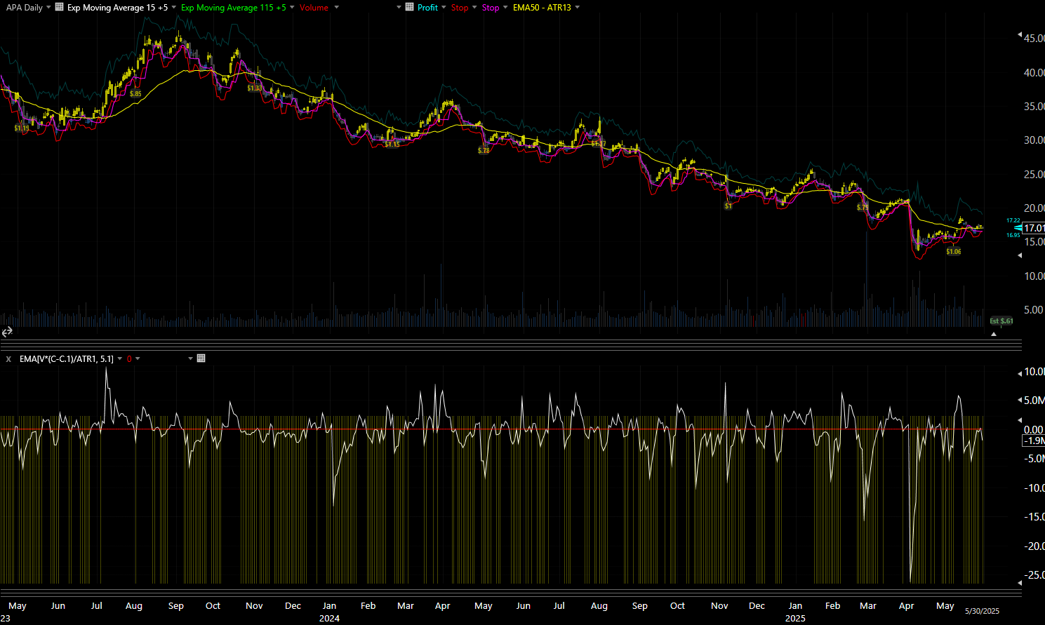
Figure 3.1.f — This chart visualizes the condition EMA[(V × (C − C.1)) / ATR[TR, 1], 5.1] > 0 applied to APA between May 2023 and April 2025.
The yellow bars in the lower panel indicate periods when the signal is active—i.e., when upward price changes are supported by rising volume and normalized against short-term volatility.
Notice how this condition frequently aligns with the initiation of directional moves—not only confirming breakouts during bullish reversals but also validating strength during sustained rallies. Equally important is its ability to filter out weaker momentum phases, reducing the risk of premature or low-conviction entries during sideways or whipsaw conditions.
Throughout the period shown, the signal demonstrates clear responsiveness to both subtle and pronounced shifts in market behavior, reinforcing its utility as a real-time momentum confirmation tool. In most system configurations, this condition would deliver the greatest value when required to be True, helping to validate entries with supportive volume dynamics—especially in strategies that rely on price action strength over prediction.
3.1.5 Trigger: L.1 > EMA[C, 26.1]
This condition evaluates whether the low of the previous day (L.1) stayed above the 26-day Exponential Moving Average (EMA) of the closing price. In systematic trading, this serves as a trend structure filter, helping to confirm that price action is not just directionally aligned but also respecting dynamic support.
When this condition is true, it suggests that the current market regime is exhibiting strength and resilience, with pullbacks finding support above a mid-range trend benchmark. It reflects a degree of trend maturity, often appearing during stable, extended bullish phases where buying pressure has absorbed short-term volatility.
However, there’s a critical nuance to consider. The condition may signal stability, but it also implies that a portion of the upward move has already occurred. This makes it potentially less favorable for short-term or early-stage entries, where better risk-reward ratios often come from buying under the support, not far above it.
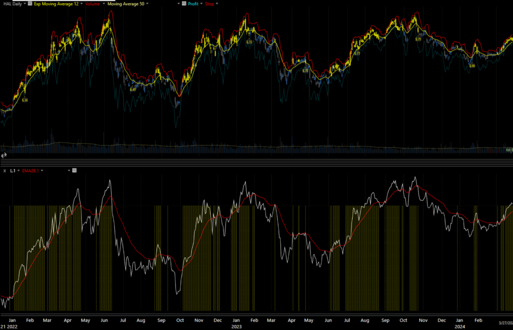
Figure 3.1.g — Visualizing the Condition on Halliburton (HAL)
This chart tracks the condition L.1 > EMA[C, 26.1] on Halliburton (HAL) from January 2022 through March 2024. Yellow bars below the price chart indicate periods when the condition is true.
Notice how the signal often clusters during sustained uptrends, coinciding with periods where the stock consistently respects dynamic support levels. These segments typically align with well-established bullish phases, where the system could benefit from longer holding times and stable entries. Meanwhile, in more volatile or sideways markets, the condition frequently toggles, reducing its effectiveness as a standalone trigger and highlighting the importance of pairing it with complementary filters.
This reinforces the condition’s role as a trend confirmation tool—best used in systems where stability and maturity of the move are more valuable than catching the earliest possible turn.
3.1.6 Trigger: L.1 > EMA[C, 13.1] + ATR[TR, 13.1]
This condition evaluates whether the previous day’s low (L.1) is positioned above a dynamically calculated threshold—specifically, the sum of the 13-day Exponential Moving Average (EMA) of the closing price and the 13-day Average True Range (ATR). This composite level serves as a volatility-adjusted upper band that reflects both the prevailing price trend and recent market turbulence.
When price action sustains itself above this upper band, it typically suggests a temporary overextension—a phase where bullish momentum may be waning, and the risk of mean reversion increases. In this context, the signal acts more as a warning flag than an invitation to enter.
Strategic Application:
- In long-only systems, this condition is rarely used as a direct trigger. Instead, it often functions best when required to be False, effectively filtering out trades that occur at potentially unsustainable highs.
- The logic is straightforward: trades initiated at these overextended levels tend to carry higher downside risk and diminished follow-through potential. By avoiding them, a system improves its entry positioning and drawdown profile.
That said, this condition shares conceptual ground with the previously discussed L.1 > EMA[C, 26.1] rule. Both aim to validate price positioning relative to trend strength, but this condition includes an added volatility buffer—making it more suitable for shorter-horizon systems that seek to avoid tops rather than ride long-lasting trends.
In practice, I rarely include both filters in the same strategy. Instead, I select based on:
- The system’s average holding period
- Its desired trade sensitivity
- Whether it’s targeting continuation trades or pullback entries
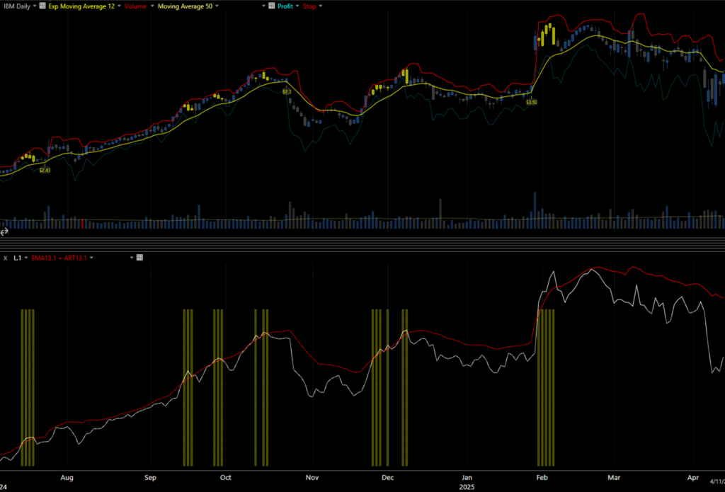
Figure 3.1.h — Visualizing the Condition on IBM (July 2024 – April 2025)
This chart applies the condition L.1 > EMA[C, 13.1] + ATR[TR, 13.1] to IBM, spanning the period from July 2024 to April 2025. Yellow bars denote periods when the condition evaluates to True—highlighting times when the prior day’s low exceeded the trend-plus-volatility threshold.
Take note of how these signals cluster near local highs, often preceding minor pullbacks or consolidations. The visual pattern confirms this rule’s strength as an exhaustion filter—one that consistently flags areas of diminishing upside potential.
By removing trades that occur during these flagged zones, a system can sharpen its edge, reduce exposure to overbought risk, and better time its entries closer to support levels.
3.1.6 Trigger: L.1 > EMA[C, 13.1] + ATR[TR, 13.1]
This condition defines a discrete, rule-based bearish reversal signal. Unlike continuous indicators like moving averages or MACD, this is a Boolean trigger—it either evaluates as true or false—based on a specific three-day price action sequence.
Pattern Logic:
- H.1 > H.2 — Today’s high is higher than yesterday’s high, showing a potential extension.
- C < C.2 — Today’s close is below the close from two days ago, suggesting momentum loss.
- H.2 > H.3 — Yesterday’s high was above the high from three days ago, indicating a temporary top formation.
When all three conditions align, the signal suggests that price has made a short-term peak, and downside movement may be imminent. It typically fires just before corrections or retracements, offering excellent utility for exit timing, hedging, or avoiding premature entries in long-only systems.
I originally encountered this elegant formation through Kerry Lovvorn on SpikeTrade.com, a platform known for tactical, pattern-driven trading methods. While deceptively simple, the rule captures subtle momentum shifts often missed by lagging indicators, giving it an edge in fast-moving or uncertain markets.
In the context of this strategy development exercise, I’ve repurposed the trigger by requiring it to be False—thereby disqualifying trades that occur just before these bearish reversals. This approach allows a long-only system to incorporate contrarian pattern recognition as a risk-avoidance mechanism, improving entry timing without adding predictive complexity.
Figure 3.1.i — AMD Three-Bar Reversal Pattern (July 2024 – April 2025)
This chart visualizes the condition H.1 > H.2 AND C < C.2 AND H.2 > H.3 on AMD, spanning from July 2024 to April 2025. Vertical yellow bars below the chart indicate when the condition is True—flagging zones where price formed a local top or shifted sharply downward soon after.
Notice how the signal repeatedly appears just before pullbacks, helping to anticipate and avoid deteriorating conditions. For long-only systems, these flags are intentionally excluded from valid entry windows, refining the overall entry profile and protecting against poor trade timing.
By integrating this type of logic—even when inverted—a systematic trader can add an extra layer of robustness to strategy design. It serves as a compelling example of how discretionary pattern insights can be effectively encoded into objective, rule-based systems.
3.2 Exit Logic: Structuring Risk and Capturing Opportunity
To ensure each strategy variant in this study remains both realistic and risk-aware, every system is equipped with a layered, rules-based exit framework. This design balances the need to protect capital with the objective of maximizing profit—without relying on discretionary intervention.
The exit model consists of three integrated components:
- Profit Target
- Hard Stop (Stop Target)
- Trailing Stop
Each element is calculated using recent price data and volatility measures, ensuring that the exit behavior adapts fluidly to shifting market conditions. Here’s a breakdown of how each is constructed and why it matters.
3.2.1 Profit Target – Volatility-Adjusted Upside Capture
Profit targets are set by adding a multiple of the 13-day Average True Range (ATR) to a recent closing price. The ATR serves as a proxy for current market volatility, and using it as a dynamic multiplier ensures that profit expectations scale with the environment.
In high-volatility regimes, the target expands, allowing room for trades to develop.
In calmer markets, it tightens, preventing overextension.
This mechanism avoids the rigidity of static price targets and keeps the system grounded in present conditions—a critical factor for swing trading strategies where range expansion matters.
By the way, I’d love to hear about the exit strategies you use. If any of them align with my approach, I’d be happy to explore and potentially feature them in future posts, so please share.
3.2.2 Hard Stop – Structural Risk Control
To protect against downside risk, each trade features a dynamic stop-loss, calculated as:
Lowest low over the past 3 days minus 13-day ATR
This approach blends short-term support structure with a medium-term volatility buffer, providing a more intelligent safety net. Unlike arbitrary fixed stops, this method allows for normal fluctuations while stepping out of the way when meaningful breakdowns occur.
It reduces the chance of being shaken out by noise,
while maintaining a disciplined exit if the setup fails.
3.2.3 Trailing Stop – Locking in Gains Over Time
To preserve open profits while allowing trades to run, a rule-based trailing stop is also integrated. It activates when:
Today’s low is higher than the low from four days ago
Once triggered, it recalculates the trailing stop as:
Lowest low over the past 6 days (excluding today) plus 23-day ATR
This adaptive trailing method encourages position longevity—it doesn’t allow winning trades too much space to breathe—but it also steps in decisively when momentum starts to fade.
Why This Exit Model Works
What makes this framework powerful is not just the individual rules, but how they work together as a system:
- The Profit Target captures potential upside with flexibility.
- The Hard Stop limits losses based on market structure.
- The Trailing Stop ensures that gains are realized as trends evolve.
Through extensive backtesting, this layered exit logic consistently outperformed single-rule systems in both stability and return metrics. It adds a structured, data-driven layer of risk and reward calibration—critical for automated or semi-automated strategies where execution decisions must be clear, repeatable, and emotion-free.
In essence, the exit system transforms a static trade idea into a dynamic lifecycle model—one that is capable of adapting, protecting, and optimizing across varied market environments.
4. Strategy Output & Performance Metrics
For each strategy variation tested, the system produces both detailed trade data and a comprehensive summary of performance. This output is designed to enable precise evaluation and comparison across thousands of condition sets – supporting both high-level insights and granular trade-level analysis.
Each individual strategy configuration generates:
- A trade log listing every position taken, including:
- Ticker symbol
- Date of entry and exit
- Entry and exit prices
- Reason for exit (profit target, hard stop, trailing stop)
- Return on trade
- Duration held
- A global summary sheet aggregating all key metrics across every tested combination. This allows rapid sorting, filtering, and performance ranking to identify the most promising strategy setups. The performance summary includes the following metrics:
- Strategy Combination ID – Unique identifier for the condition set (e.g., “1020121”)
- Total Number of Trades – Count of executed positions over the backtest period
- Total Return – Net percentage gain or loss over all trades
- Return per Trade – Average return per position, including both winners and losers
- Batting Average (Win Rate) – Proportion of trades closed in profit
- Average Holding Time (All Trades) – Overall average time in trade
- Average Holding Time (Winners Only) – Duration of successful trades
- Average Holding Time (Losers Only) – Duration of losing trades
- Average Time to Profit Target – Days taken, on average, to reach the target price
- Average Time to Stop Loss – Days to reach the hard stop
- Average Time to Trailing Stop – Days until exit via trailing logic
- Total Value Gained – Aggregate profit across all winning trades
- Total Value Lost – Aggregate loss across all losing trades
- Number of Winning Trades
- Number of Losing Trades
- Maximum Return per Trade – Largest single-trade gain
- Maximum Loss per Trade – Largest single-trade loss
- Average Return per Winning Trade
- Average Loss per Losing Trade
- A trade log listing every position taken, including:
This structured output ensures that no detail is overlooked and that each strategy’s strengths and weaknesses can be quantitatively assessed. Ultimately, it enables clear, data-driven decisions in the development of robust, tradable systems.
Why This Matters
While headline metrics like total return or win rate are important, they rarely tell the full story. The real strength of this analytical framework lies in its ability to reveal how each strategy behaves over time—uncovering patterns of consistency or volatility that determine whether a system is structurally reliable or merely a statistical illusion.
In past research, I’ve frequently encountered strategies with exceptional backtested results—on paper. But closer examination often revealed a fragile foundation: their performance was clustered within narrow timeframes, thriving during specific market regimes only to break down completely when conditions shifted. For example, a system might post excellent gains in the first half of a two-year test, then stagnate—or even decline—throughout the second half. This kind of lopsided behavior raises serious concerns about overfitting and adaptability.
To avoid falling into that trap, I deconstruct each strategy’s performance across multiple dimensions—temporal segments, exit mechanics, trade duration, and outcome distribution. This helps me quickly identify false positives: strategies that appear strong due to timing luck rather than intrinsic resilience. On the other hand, those that maintain consistent results across varied conditions become prime candidates for deeper refinement and real-world application.
This level of scrutiny transforms a promising backtest into something potentially tradable. It shifts the focus from raw numbers to what actually matters: durability, repeatability, and compatibility with real-market dynamics.
4.1 Backtest Results
Once the strategy logic was finalized, I integrated it into my research platform and launched a full-scale backtest. This process ran continuously for approximately one week—evaluating thousands of strategy permutations across over 200 tickers, using two full years of historical market data. While the system crunched through the combinations, I also used the time to consider how to best structure this post. If you find any section helpful—or unclear—I genuinely welcome your feedback. Please feel free to leave a comment or reach out privately. Your input will help me improve and refine this series.
Now, let’s dive into the results.
When assessing system performance, I focus initially on three core metrics:
- Total Return – to quantify absolute profitability over the test period.
- Return per Trade (RpT) – to evaluate the efficiency and average value of each trade.
- Total Number of Trades – to ensure there’s sufficient data to draw meaningful conclusions, while also checking that the strategy remains operationally manageable.
Together, these three indicators provide a practical lens through which to evaluate strategy viability. I’m not only looking for strategies that are profitable on paper—I’m looking for those that are realistically tradable. Systems should generate enough trades to validate their performance statistically, but not so many that they require impractical levels of automation or oversight.
Of course, the temptation is always to jump directly to the top performers by total return. And while those outliers often deliver eye-catching results, they rarely represent the most reliable candidates for live deployment. More often than not, they turn out to be overfit configurations—strategies that happened to thrive within the specific backtest window but lack robustness across varying market conditions.
That said, these high-return combinations still serve a critical purpose. They help define the performance ceiling—the upper limit of what’s theoretically possible under ideal circumstances. By examining these outliers, I can better understand which conditions and indicator combinations have the most latent potential, even if they’ll need to be tempered or refined before practical use.
The table below outlines key statistics from the highest-returning strategy configurations, providing a reference point for what worked best in this specific environment.
Binary Code | Trades | Total Return (%) | Return per Trade (RpT%) | Batting Average (%) | Avg. Holding Time |
0000002 | 14,674 | 2025.88 | 0.1381 | 52.89 | 8.2 days |
0000022 | 14,332 | 2004.09 | 0.1398 | 52.99 | 8.0 days |
0000000 | 14,911 | 1996.81 | 0.1339 | 52.74 | 8.1 days |
0002002 | 12,168 | 1989.24 | 0.1635 | 55.18 | 7.9 days |
0002000 | 12,348 | 1987.55 | 0.1610 | 55.29 | 7.9 days |
0002022 | 12,095 | 1975.97 | 0.1634 | 55.18 | 7.9 days |
0000020 | 14,543 | 1970.86 | 0.1355 | 52.85 | 7.9 days |
0002020 | 12,267 | 1962.84 | 0.1600 | 55.27 | 7.9 days |
0020002 | 12,170 | 1829.57 | 0.1503 | 55.14 | 7.9 days |
0020000 | 12,899 | 1821.66 | 0.1412 | 54.38 | 7.7 days |
Table 4.1.a — Top 10 Strategy Variants by Total Return
This table highlights the top 10 strategy combinations based on total return, as tested across 200 U.S. equity tickers over a two-year historical window starting in 2023.
While these strategies achieved the highest cumulative returns within the test universe, they may not necessarily be viable for real-world trading in their current form. Many exhibit modest Return per Trade (RpT) figures and only moderate Batting Averages (win rates). These metrics suggest that while total return is high, the efficiency and reliability of each trade may not meet the standards required for practical implementation—especially for risk-conscious traders.
Still, these results are valuable. They offer a reference point for what’s achievable under ideal historical conditions and provide clues about the types of indicator configurations that have the potential to deliver outsized gains. Used thoughtfully, these combinations can inform the development of more stable and operationally sound systems by serving as benchmarks for both opportunity and caution.
From these results, one key insight becomes apparent: the exit logic appears to be well-calibrated. Even the most basic system—represented by the code 0000000, which simply enters a trade each day that no position is open for a given ticker—yielded a positive return. Unsurprisingly, this variation also executed the highest number of trades, reflecting its always-on entry behavior without any filtering logic.
This further reinforces the importance of the exit structure. Even without sophisticated entry criteria, the strategy was able to deliver gains by relying solely on the strength of its stop-loss, trailing stop, and profit target mechanics.
Another noteworthy observation is that most of the top-performing systems likely benefited more from trade frequency than from intricate logic design. None of the top 10 configurations appear especially complex—most use minimal filtering, but I identify a strong pattern of systems relying heavily on conditions set to “2” (i.e., requiring a trigger to be false). With that said, that might mean such conditions can play a critical role in final system development—as they did dominate in this early return-based ranking.
In short, the strong total returns shown here seem to be driven primarily by volume of trades, rather than by precision or sophistication of signal logic. This provides useful context moving forward: to build a robust, scalable system, I’ll need to strike a better balance between selectivity and trade frequency—hopefully maximizing efficiency without sacrificing consistency.
4.1.1 Understanding the Perspective
To ensure a realistic and risk-conscious evaluation, each strategy in the backtest was configured to risk exactly 1% of the portfolio per trade. As a result, the figures shown in the “Total Return” column represent cumulative gains relative to the initial portfolio value. For example, a return of 2026% means that the strategy grew the portfolio by 20.26 times over the two-year testing period.
While those results may appear exceptional at first glance, total return is not my primary decision-making metric—and it shouldn’t be. Without the proper context, it can be misleading. Here’s why:
A strategy might generate a large total return simply because it executed a very high number of trades, each yielding a small profit. That may look great in backtest summaries, but in reality, it could translate into operational chaos—requiring a trader to manage hundreds of marginal trades with tight timing windows and little edge per trade.
Even more concerning is when a strategy’s performance is front-loaded—making most of its gains early in the testing period, then stalling or declining later. This pattern can be corrected, but most likely it will require overfitting, where the system will capture favorable market conditions that are unlikely to persist.
Because of these risks, I place significant weight on Return per Trade (RpT). It’s not just a profitability metric—it’s a proxy for system efficiency. A high RpT suggests that each trade contributes meaningful returns, which is critical for real-world application, especially for discretionary traders or those with limited execution bandwidth.
It’s also important to note that total return tends to correlate with trade count—more trades mean more compounding, but also greater exposure to noise. That’s why I focus on systems that strike a balance between profitability and manageability.
For me, RpT is one of the clearest signals of that balance. It helps identify strategies that don’t just make money, but do so consistently, cleanly, and in a scalable way.
That said, Return per Trade (RpT) is not without its limitations. A high RpT can occasionally be skewed by a small number of outlier trades with exceptional returns, artificially inflating the average. However, in this particular analysis, the likelihood of such distortion is minimal. Given that the exit conditions were intentionally designed to be conservative—with tight profit targets, disciplined stop-losses, and volatility-based trailing exits—it’s unlikely that any one trade could disproportionately impact the overall average. As a result, the RpT in this case can be interpreted as a more reliable measure of trade efficiency.
Trades | Binary | Return | RpT | B.A | Average Holding Time |
24 | 0122011 | 11.9 | 0.4957 | 75 | 8.7 days |
24 | 2122011 | 11.9 | 0.4957 | 75 | 8.7 days |
24 | 0122111 | 11.9 | 0.4957 | 75 | 8.7 days |
24 | 2122111 | 11.9 | 0.4957 | 75 | 8.7 days |
18 | 1100011 | 8.49 | 0.4717 | 61.11 | 7.2 days |
18 | 1120011 | 8.49 | 0.4717 | 61.11 | 7.2 days |
18 | 1101011 | 8.49 | 0.4717 | 61.11 | 7.2 days |
18 | 1121011 | 8.49 | 0.4717 | 61.11 | 7.2 days |
18 | 1100111 | 8.49 | 0.4717 | 61.11 | 7.2 days |
18 | 1120111 | 8.49 | 0.4717 | 61.11 | 7.2 days |
Table 4.1.b — This table showcases the top 10 strategy combinations ranked by Return per Trade (RpT) across 200 tickers during the 2023–2025 backtest period.
Each was evaluated using a contradictions filter to ensure internal logical consistency. These results highlight the most efficient systems—those that generate the highest average return per trade—making them prime candidates for real-world implementation where trade quality and manageability matter more than sheer volume.
4.1.2 Analyzing Return per Trade (RpT) vs. Trade Volume
One of the recurring patterns I’ve observed—both in this study and throughout prior research—is the inverse relationship between Return per Trade (RpT) and total trade volume. Strategies with the highest RpT often execute relatively few trades. While these systems can appear highly efficient on a per-trade basis, this low frequency introduces a critical limitation: statistical fragility due to limited sample size.
Even if a low-trade-count strategy reports impressive metrics—high RpT, a solid batting average, and favorable holding durations—it remains difficult to trust those results without broader validation. A system that has only produced a few dozen or even a few hundred trades may be reflecting a lucky fit to a specific historical context rather than a structurally sound, repeatable edge.
This is why I treat such systems with healthy skepticism. They may look appealing in isolation, but their practical risk is much higher. The danger is particularly acute when the strategy’s performance hinges on rare price structures or one-off market conditions that are unlikely to recur in live trading.
My focus is on identifying systems that strike a measured balance between efficiency (RpT) and reliability (trade volume). A system that performs consistently across a large number of trades is far more likely to retain its edge across different market environments. And from a trader’s standpoint, it’s much easier to trust and scale a system that proves itself over time with a statistically meaningful sample.
As I continue refining and filtering my results, this balance remains a core criterion: I aim to select strategies that are not only profitable, but sustainable, both in their statistical characteristics and their operational demands.
Trades | Binary | Return | RpT | B.A | Avg Holding Time |
265 | 1220010 | 78.47 | 0.2961 | 56.23 | 10.9 days |
265 | 1221010 | 78.47 | 0.2961 | 56.23 | 10.9 days |
301 | 1020110 | 88.61 | 0.2944 | 57.48 | 10.6 days |
301 | 1021110 | 88.61 | 0.2944 | 57.48 | 10.6 days |
303 | 1020010 | 88.77 | 0.293 | 57.43 | 10.6 days |
303 | 1021010 | 88.77 | 0.293 | 57.43 | 10.6 days |
96 | 1200011 | 27.75 | 0.289 | 55.21 | 8.4 days |
96 | 1220011 | 27.75 | 0.289 | 55.21 | 8.4 days |
96 | 1201011 | 27.75 | 0.289 | 55.21 | 8.4 days |
Table 4.1.c — This table visualizes the top 9 strategy combinations that best balance Return per Trade, total return, and trade frequency, as tested across 200 U.S. tickers from 2023–2025. By filtering out low-sample outliers, it highlights systems with a more sustainable performance profile—offering a strong mix of profitability, statistical robustness, and real-world viability.
4.1.3 A Balanced System Example
Among the top-performing candidates identified during this analysis, one system stood out for its well-rounded balance of profitability, simplicity, and operational manageability. This configuration—known by its binary identifier 1020010—maintains a moderate trade volume that is low enough to remain manageable in practice, yet sufficiently high to support meaningful statistical inference. It offers strong returns without relying on overly complex logic or overfitting to past data.
Interestingly, several closely related systems—specifically 1020110, 1021110, 1020010, and 1021010—delivered nearly identical performance. Each employs a slightly different combination of logical triggers drawn from the same set of conditions. I chose to highlight 1020010 because of its structural clarity: it activates fewer conditions while still achieving strong results. Most of its trigger states are set to 0, meaning they are inactive or excluded. This minimalism reduces logical conflicts, lowers the risk of over-optimization, and makes the system easier to interpret, implement, and maintain.
4.1.4 Logic Composition of System 1020010
Below is a breakdown of the specific triggers used in this configuration, along with their functional descriptions:
|
Trigger |
Bin |
Evaluated Result |
|
EMA[C, 27] > EMA[C, 17]
|
1 |
True |
|
EMA[C, 115.5] – EMA[C, 15.5] < ATR[TR, 65.5] * 0.6
|
0 |
N/A |
|
MACD[C, 7.15.5] > MACD[C.1, 7.15.5]
|
2 |
False |
|
EMA[(V * (C – C.1)) / ATR[TR, 1], 5.1] > 0
|
0 |
N/A |
|
L.1 > EMA[C, 26.1]
|
0 |
N/A |
|
L.1 > EMA[C, 13.1] + ATR[TR, 13.1]
|
1 |
True |
|
H.1 > H.2 AND C < C.2 AND H.2 > H.3
|
0 |
N/A |
Only three out of seven triggers are actively evaluated in this system (Bin ≠ 0). Among these, two returned True and one returned False, while the remaining four were excluded (N/A). This simplicity is a strength, not a limitation—it ensures that the system remains focused on a small, well-performing subset of conditions, reducing cognitive overhead and simplifying both live tracking and future refinements.
By emphasizing clear logic over brute-force complexity, System 1020010 achieves the kind of practical robustness I look for in a strategy. It’s a prime example of how strong results can emerge from thoughtful design rather than maximalist configuration.
4.1.5 System Overview and Trade Triggers
The 1020010 system is built around a streamlined trio of entry conditions—striking a careful balance between simplicity, interpretability, and performance. It activates trades only when the following criteria are met:
- EMA[C, 27] > EMA[C, 17]
A medium-term trend alignment filter that signals bearish momentum. When the longer EMA is above the shorter one, it suggests a declining price structure—indicating that the asset is in a corrective or distributional phase. - MACD[C, 7.15.5] < MACD[C.1, 7.15.5]
A short-term momentum softening signal. This condition detects early-stage weakness—typically occurring when upside momentum begins to stall, often just before a mean reversion or pullback. - L.1 > EMA[C, 13.1] + ATR[TR, 13.1]
A volatility-adjusted threshold designed to identify price overextensions. When the previous day’s low exceeds this dynamic upper band, it often reflects unsustainable upward pressure—highlighting setups that are ripe for short-term reversion.
- EMA[C, 27] > EMA[C, 17]
Individually, each rule plays a distinct role: trend filtering, momentum timing, and volatility normalization. Combined, they form a cohesive framework designed to exploit tactical pullbacks within broader downtrends—identifying moments where price strength appears overextended and structurally vulnerable..
Since the strategy operates on daily closing prices, optimal execution occurs near the end of the trading session. This ensures the backtested logic aligns with live implementation and minimizes slippage between signal generation and order execution.
In the next section, we’ll examine the actual trade log generated by this system. This dataset includes detailed metrics such as entry/exit timing, trade duration, and realized returns—offering valuable insight into whether this system maintains its structural edge in practice and is suitable for further optimization or live deployment.
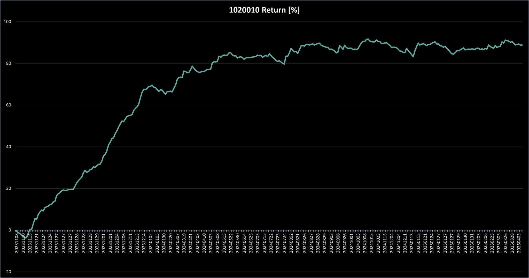
Figure 4.1.a — System 1020010: Return Over Time (2023–2025)
This chart displays the cumulative return profile for strategy 1020010 applied across 200 U.S. equities over a two-year period. Notably, the system demonstrates a strong initial uptrend through 2023, followed by a more stable consolidation phase throughout 2024 and into early 2025. The smooth upward curve prior to January 2024 suggests high-quality trade execution, while the flattened slope that follows indicates diminished opportunity density—an important consideration for ongoing refinement.
5. System Performance Review
At first glance, the system’s equity curve paints an optimistic picture: consistent upward movement, particularly during the initial months of the backtest. However, a deeper analysis reveals a critical flaw—the vast majority of gains occurred before January 2024, with performance plateauing thereafter.
Over the full two-year test period, the system executed 303 trades, a modest number that limits statistical confidence. Notably, a significant concentration of trades and profits occurred during late 2023. Post-January 2024, both trade frequency and profitability declined sharply.
To assess this shift more clearly, I segmented performance into two key timeframes.
Performance Breakdown
Nov 2023 – Jan 2024:
- Total Return: 68.94%
- Profit per Trade (PrT): 0.386
- Number of Trades: 80
Jan 2024 – Apr 2025:
- Total Return: 19.83%
- Profit per Trade (PrT): 0.089
- Number of Trades: 152
Despite nearly doubling the number of trades in the latter period, performance deteriorated sharply. Based on the pace set in late 2023, one would have expected roughly 640 trades over the second window. Instead, execution dropped by 76%, and both total return and efficiency (as measured by RpT) fell by over 70%.
This stark contrast suggests that the system’s early success was likely driven by favorable—possibly unique—market conditions, rather than a structurally sound strategy. The significant drop-off in both output and efficiency implies fragility and limited adaptability to evolving environments.
Conclusion
While the system initially showed promise, its inability to sustain performance makes it unsuitable for further development. In trading system design, consistency across time is paramount. A system that thrives only during isolated conditions is likely overfit and unsuitable for live deployment.
With that in mind, I’ll now shift focus to evaluating the next candidate—looking for stronger signals of robustness and repeatability.
5.1 Moving Forward: A Potentially Better System
Trades | Binary | Return | RpT | B.A | Average Holding Time |
565 | 0220012 | 138.2 | 0.2446 | 56.11 | 11.0 days |
564 | 0220112 | 137.85 | 0.2444 | 56.03 | 11.0 days |
312 | 1200010 | 76.11 | 0.2439 | 56.73 | 11.7 days |
312 | 1201010 | 76.11 | 0.2439 | 56.73 | 11.7 days |
690 | 1220102 | 168.1 | 0.2436 | 53.48 | 9.1 days |
148 | 0122012 | 35.78 | 0.2418 | 64.86 | 8.2 days |
148 | 2122012 | 35.78 | 0.2418 | 64.86 | 8.2 days |
148 | 0122112 | 35.78 | 0.2418 | 64.86 | 8.2 days |
148 | 2122112 | 35.78 | 0.2418 | 64.86 | 8.2 days |
Table 5.1.a — Strategy combinations ranked 126–134 by overall Return per Trade (RpT). These candidates also maintain a healthy balance between total return and trade count, suggesting a combination of efficiency and structural soundness.
As I continue through the ranked combinations, System 1220102 stands out as a promising next candidate. Not only does it deliver a high total return, but it also maintains a respectable Return per Trade (RpT) and a solid batting average (B.A.) – a combination that suggests both efficiency and consistency.
What makes this system especially interesting is its similarity to the previous model. Two of its three entry conditions overlap with the underperforming system we just reviewed. This presents an opportunity: by comparing the structures and outcomes of both, I may be able to identify repeatable patterns or distinguishing features that separate high-quality signals from weaker ones.
This analysis could reveal whether certain trigger combinations are more robust across different market regimes or if specific conditions consistently degrade performance. If the positive characteristics seen in 1220102 hold up under scrutiny, it may serve not only as a viable trading system on its own, but also as a blueprint for future system development.
With that in mind, I’ll now shift focus to a deeper evaluation of this configuration – examining trade behavior, performance over time, and the interactions between its triggers. The goal is to determine whether this system offers a structurally sound, repeatable edge, or if it too falls into the category of temporary success driven by specific market phases.
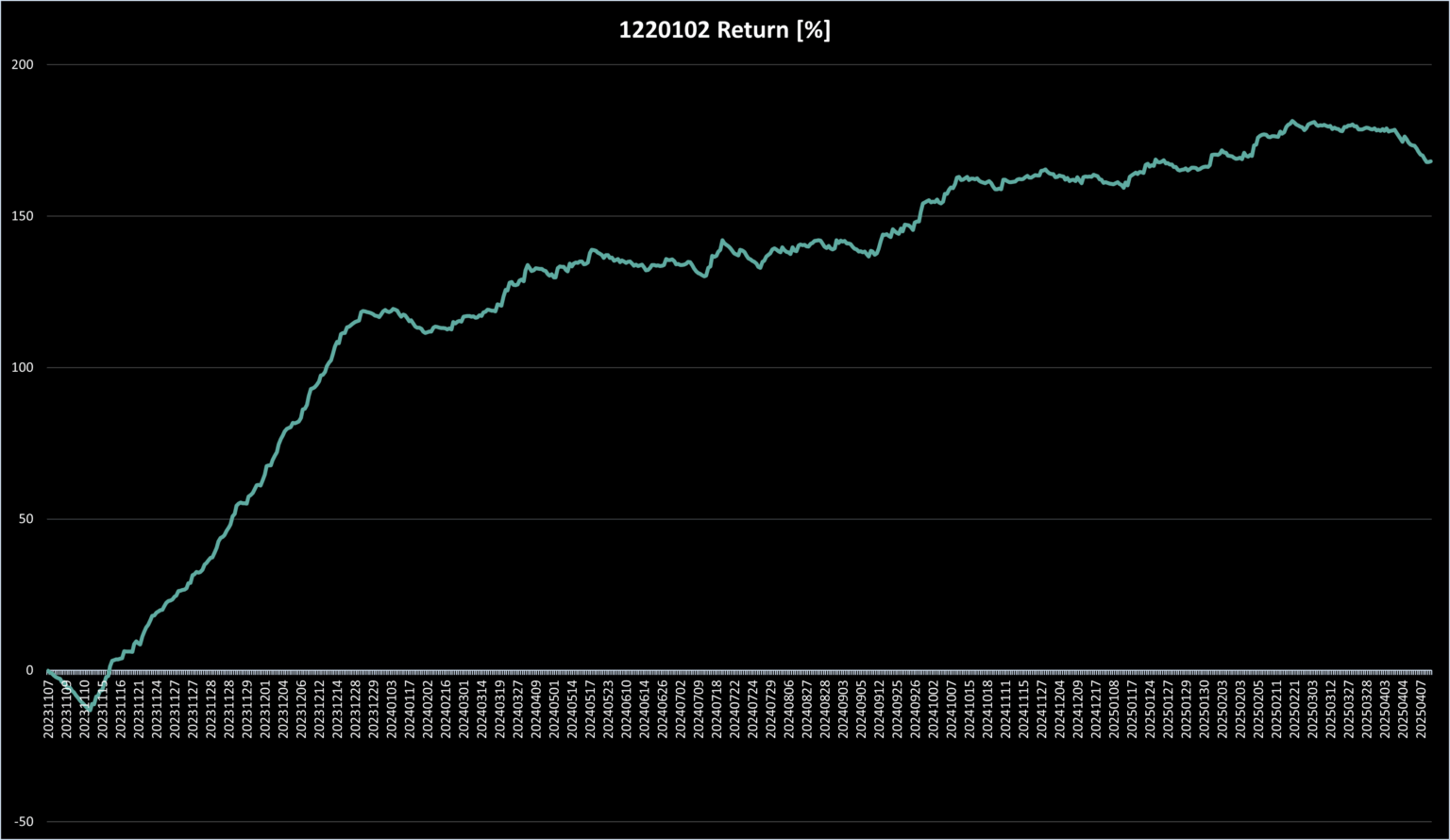
Figure 5.1.a — Equity Curve for System 1220102
This chart tracks the cumulative return of System 1220102 over a two-year backtest across 200 U.S. equity tickers. The system generated strong absolute returns while maintaining a remarkably consistent upward trajectory—a promising sign of structural integrity.
What stands out is not just the height of the curve, but its shape: a steady climb with limited drawdowns, minimal stagnation, and sustained performance through early 2025. This reflects the system’s ability to convert time into profit efficiently, a key advantage for swing and systematic traders seeking to optimize capital turnover and reduce idle exposure.
There are brief periods of consolidation and mild pullbacks—especially toward the final months—but no prolonged breakdowns. This suggests that the system was adaptive across multiple market conditions, rather than overly reliant on a single regime or short-lived pattern.
As we move forward, I’ll dissect the underlying trade structure and time-segmented results to determine whether the performance shown here is repeatable and robust, or if it’s potentially masking weaknesses that could emerge under different market dynamics.
5.1.1 System Performance Breakdown: 2023 vs. 2024
To evaluate the structural reliability of System 1220102, I segmented its performance across two distinct timeframes: the initial launch phase during the final two months of 2023, and the follow-up stretch spanning all of 2024 through April 2025. The goal was to assess not just whether the system generated profit, but whether it could maintain consistency as market conditions evolved.
5.1.2 Performance Summary
November–December 2023:
- Total Return: 118.81%
- Profit per Trade (PrT): 1.485
- Number of Trades: 168
January 2024 – April 2025:
- Total Return: 49.29%
- Profit per Trade (PrT): 0.0944
- Number of Trades: 522
At first glance, the system continued to deliver positive returns well beyond the initial test window. That in itself is encouraging. However, the steep drop in Profit per Trade—from 1.485 to 0.0944—is significant. It raises concerns about the system’s resilience and scalability across market phases.
More trades were executed in the latter period, yet the return profile weakened noticeably. This could point to saturation, degradation of edge, or simply a shift in market character that the current configuration doesn’t adequately adapt to.
What’s important to note is that despite the performance drop, the system remained net-profitable through 2024 and into 2025. That fact alone differentiates it from many high-return systems that quickly collapse once conditions change. However, the severity of the drop-off in trade efficiency suggests that further refinement is necessary.
5.1.3 Comparative Variant Exploration
To dig deeper, I began reviewing structurally similar systems—those with minimal changes to the core logic of 1220102. Variants like 120102, 1221102, and others clustered near it in the rankings offer valuable insight. If performance differences between these systems prove consistent, I might be able to isolate which triggers are responsible for resilience—and which are more sensitive to fleeting conditions.
Below is a table showcasing some of the systems currently under review. Each was selected based on similarity to 1220102 and evaluated across the same two-year testing period on 200 U.S. tickers:
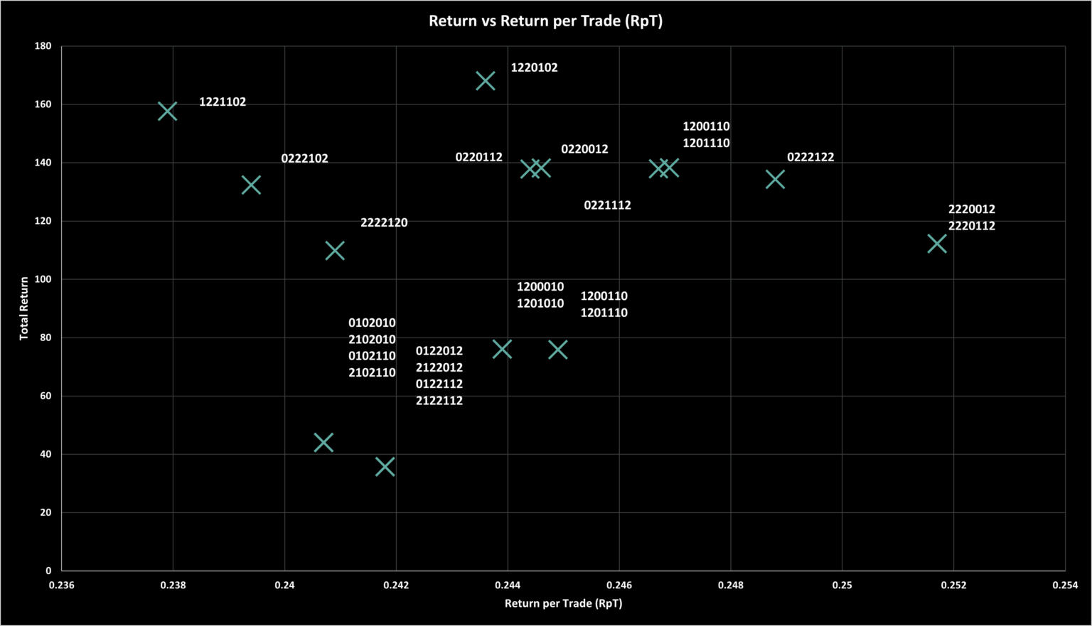
Figure 5.1.b — Strategy combinations ranked 119–141 by overall Return per Trade (RpT). These candidates also maintain a healthy balance between total return and trade count, suggesting a combination of efficiency and structural soundness.
Key Insights:
- 1220102 (center-left) has one of the highest total returns (~168%) while maintaining a moderate RpT (~0.244) — suggesting solid trade frequency and profit efficiency.
- 2220012, although slightly higher in RpT (~0.252), falls short in total return — hinting that a slightly more frequent or balanced strategy like 1220102 may scale better.
- Systems like 2122012 or 2122112 show high RpT but lower overall return due to fewer trades, which could be statistically fragile.
This comparison enables me to detect which patterns appear repeatable—and which are more likely the result of luck or unique market phases. Additionally, these data points help determine whether further parameter tuning, or even introducing a new condition, could stabilize performance across the full test period.
In the next section, I’ll dive into system 1221102 and begin breaking down how its return profile differs from 1220102—despite their structural similarities. I’ll also begin exploring whether there’s a way to close the performance gap between early-stage acceleration and long-term consistency by adjusting the entry filter logic or redefining the exit thresholds.
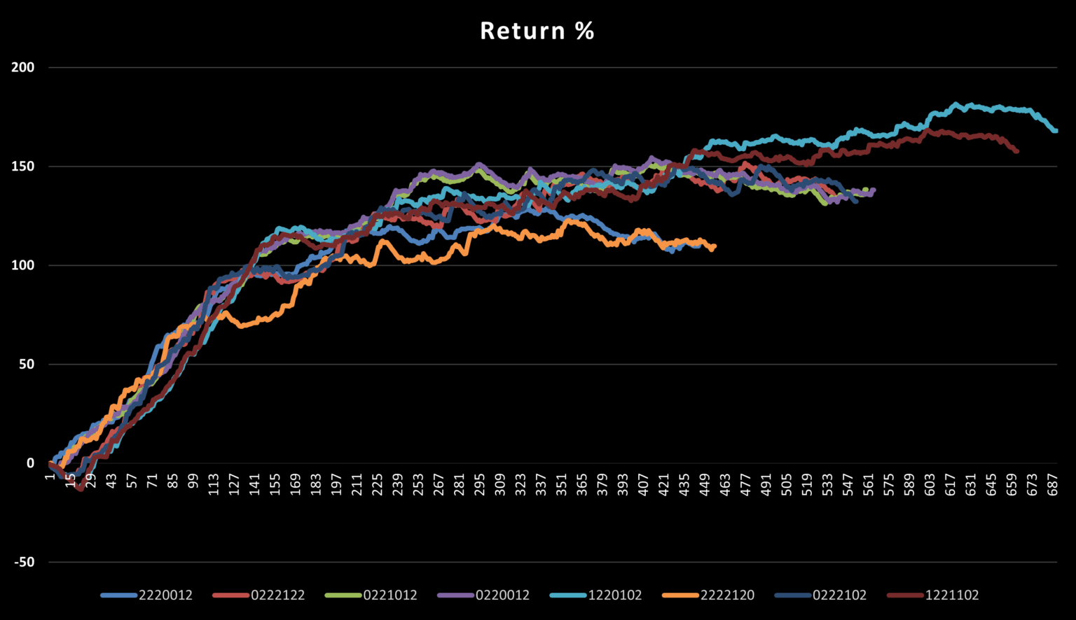
Figure 5.1.c — Strategy Combinations Ranked by Return per Trade (RpT), Positions 119–141 (selected systems)
This chart visualizes strategy variants ranked 119 through 141 by Return per Trade (RpT), offering a comparative snapshot of efficiency across this performance tier. Each point reflects a distinct configuration tested over 200 tickers in a two-year window. By mapping them on a return-per-trade axis, we gain a clearer perspective on relative trade quality—helping to identify which systems deliver consistent gains per trade, even if they don’t top the list in total return.
| 2220012 | 0222122 | 0221012 | 0220012 | 1220102 | 2222120 | 0222102 | 1221102 |
Return | 112.27 | 134.34 | 138.25 | 138.2 | 168.1 | 109.86 | 132.39 | 157.72 |
RpT | 0.2517 | 0.2488 | 0.2469 | 0.2446 | 0.2436 | 0.2409 | 0.2394 | 0.2379 |
Trades | 446 | 540 | 560 | 565 | 690 | 456 | 553 | 663 |
Table 5.1.c — Strategy Combinations Ranked 119–141 (selected systems) by Return per Trade (RpT): Evaluating the Balance Between Return, Efficiency, and Trade Volume
This table presents a curated selection of strategy combinations ranked between positions 119 and 141 by Return per Trade (RpT). The purpose of this comparison is to highlight configurations that strike a meaningful balance between three critical dimensions: total return, trade efficiency (RpT), and execution volume. Systems listed here may not deliver the absolute highest returns, but they offer structurally sound profiles—efficient enough to justify inclusion in a live portfolio, and active enough to build statistical confidence over time.
| 2220012 | 1220102 | ||||
Year | 2023 | 2024 | 2025 | 2023 | 2024 | 2025 |
Return | 95.69 | 27.76 | -11.18 | 119.01 | 41.56 | 7.53 |
RpT | 0.602 | 0.132 | -0.039 | 0.704 | 0.117 | 0.045 |
Trades | 159 | 210 | 287 | 169 | 354 | 167 |
| 0222122 | 2222120 | ||||
Year | 2023 | 2024 | 2025 | 2023 | 2024 | 2025 |
Return | 94.71 | 53.78 | -14.15 | 71.61 | 50.31 | -12.06 |
RpT | 0.631 | 0.191 | -0.131 | 0.689 | 0.195 | -0.128 |
Trades | 150 | 282 | 108 | 104 | 258 | 94 |
| 0221012 | 0222102 | ||||
Year | 2023 | 2024 | 2025 | 2023 | 2024 | 2025 |
Return | 114.88 | 28.98 | -5.61 | 96.64 | 52.39 | -16.64 |
RpT | 0.611 | 0.107 | -0.056 | 0.721 | 0.171 | -0.147 |
Trades | 188 | 271 | 101 | 134 | 306 | 113 |
| 0220012 | 1221102 | ||||
Year | 2023 | 2024 | 2025 | 2023 | 2024 | 2025 |
Return | 116.46 | 28.60 | -6.86 | 115.27 | 36.82 | 5.63 |
RpT | 0.616 | 0.105 | -0.067 | 0.703 | 0.106 | 0.037 |
Trades | 189 | 273 | 103 | 164 | 348 | 151 |
Table 5.1.d — Strategy Combinations Ranked 119–141: Year-by-Year Breakdown of Return, RpT, and Trade Volume
This table highlights selected strategy combinations ranked between positions 119 and 141 by Return per Trade (RpT), with performance data segmented by calendar year. It is structured to facilitate comparison across three key dimensions: total return, trade efficiency (RpT), and trade frequency. By dividing the metrics year by year, the table reveals how each system’s characteristics evolved over time—making it easier to identify whether the strategy maintained consistency or showed signs of deterioration or overfitting. This level of granularity is essential for evaluating long-term viability and adapting strategies to shifting market conditions.
5.2. System Comparison
To evaluate the broader context of performance sustainability, I compared System 1220102 with several closely related configurations. The results across these alternatives were telling.
Systems 2220012, 0222122, 2222120, 0221012, 0222102, and 0220012 all posted negative returns in 2025, indicating a structural breakdown or lack of adaptability in recent market conditions. Only 1220102 and 1221102 maintained positive performance into 2025.
Between the two, 1220102 appears stronger on the surface: it delivered a higher Return per Trade (RpT) and produced a larger number of trades, which translated into a higher overall return. From a raw metrics perspective, it outperformed its peer.
However, when we examine the underlying characteristics, concerns start to emerge. The RpT for the first four months of 2025 was just 3.7% for 1220102 and 4.5% for 1221102. While still positive, these numbers are well below what I consider viable – especially when annual degradation trends show that system efficiency has been declining sharply since early 2024.
Even accounting for the relatively short 2025 data sample (four months), the consistent deterioration in quality is a clear red flag. The system’s ability to generate profitable, high-quality trades appears to be eroding, suggesting that its previous success may have been tied to temporary conditions no longer present.
Conclusion: Despite the positive total return, System 1220102 fails to meet my minimum standards for reliability and efficiency, and as such, will not be considered for further development. I’ll continue exploring other candidates that exhibit stronger consistency and a healthier return profile across the entire test range.
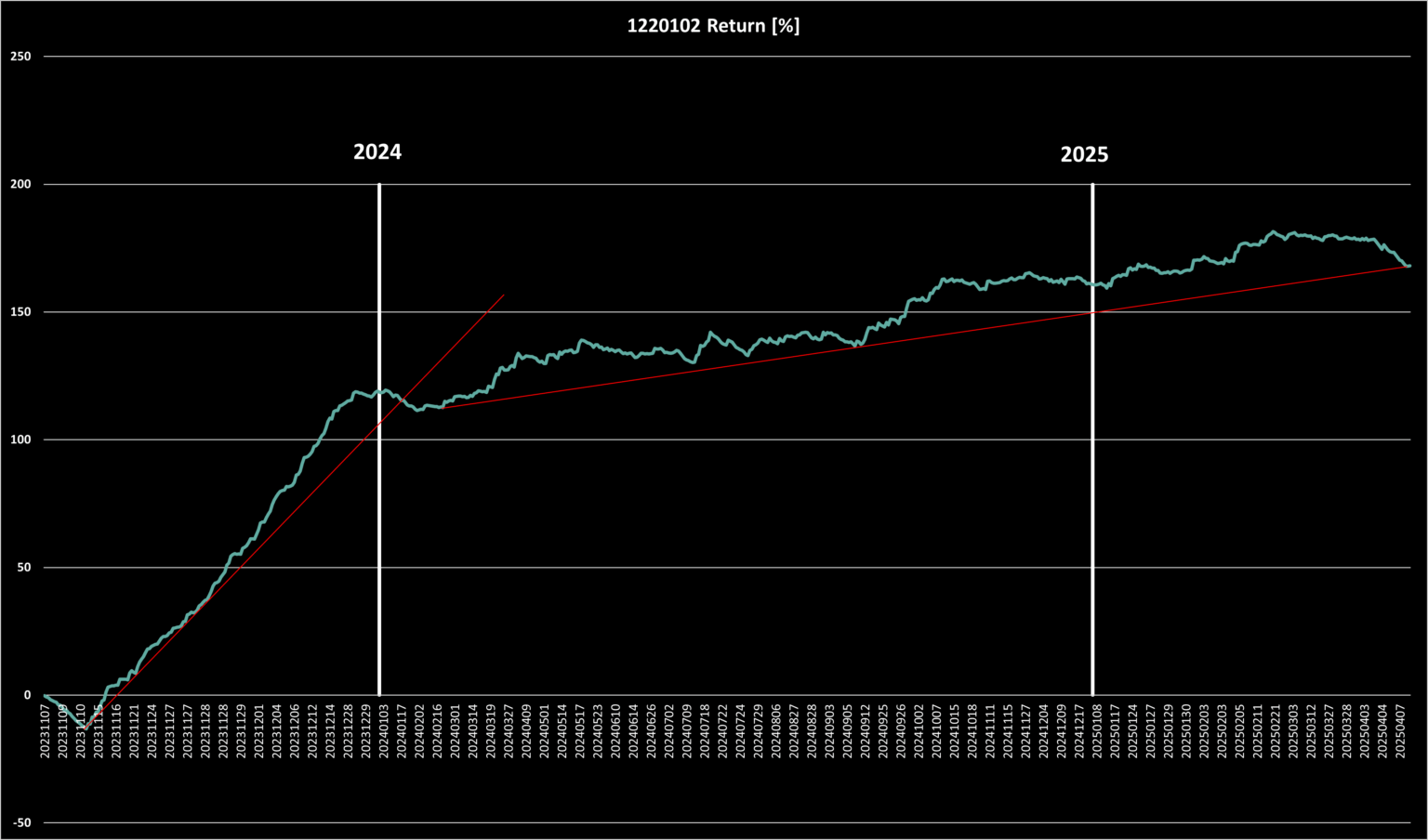
Figure 5.2.a — Equity Curve for System 1220102
This chart displays the cumulative return trajectory of System 1220102 across a two-year backtest conducted on 200 U.S. equity tickers. The equity curve reflects the system’s overall profitability and momentum across time. Red trend lines have been overlaid to emphasize a noticeable shift in performance: strong, consistent gains through the end of 2023 are followed by a more gradual and less stable growth trajectory beginning in 2024. This visual segmentation helps highlight the point at which the system’s behavior began to change, prompting a deeper investigation into whether the shift reflects a temporary regime change or a structural weakness in the system itself.
5.2.1. A New Contender: Digging Deeper Down the RpT Ladder
While scanning through the mid-tier of the Return per Trade (RpT) rankings, I encountered a system that hadn’t initially drawn attention based on total return alone—but upon closer inspection, it presents a compelling case for further evaluation. This strategy may not deliver eye-catching gains per trade, but what it offers instead is a rare blend of consistency, resilience, and manageable trade volume.
Unlike many top-return systems that saw their edge collapse in 2025, this new candidate maintained a relatively stable performance across both years of testing. It didn’t spike early and fade away—it simply kept working. That kind of quiet dependability is often more desirable than headline numbers, particularly when designing systems meant for long-term deployment.
This discovery is a useful reminder: strong systems don’t always appear at the top of the leaderboard. They often reside just below the surface—overshadowed by high-flying (and often overfit) performers. When Return per Trade, trade frequency, and temporal consistency align, even a system with moderate returns can form the foundation of a robust, scalable strategy.
To explore this possibility, I’ll now directly compare this system to System 2222120, which we previously reviewed and ultimately dismissed due to its deteriorating behavior in 2025. In the following section, I’ll unpack the entry conditions, trade characteristics, and year-over-year stability of both candidates—highlighting why this new contender might be the more viable path forward in building a durable, long-only automated framework.
5.2.3. System Comparison: 2222120 vs. 2122202
When evaluating long-term system viability, it’s important to consider not just performance highs, but how well a system holds up over time – especially across different market regimes. System 2222120 initially appeared promising due to its minimal performance fluctuation between November–December 2023 and the subsequent period through April 2025. This suggested a degree of stability not present in many other configurations.
However, a closer review of its 2025 results – now supported by nearly half a year of data – tells a different story. Despite its consistency, the system experienced a noticeable decline in performance, with diminishing return quality and trade impact. Given this trend, and the fact that its edge appears to be fading, 2222120 no longer justifies deeper exploration.
In contrast, System 2122202 emerges as a compelling alternative. While not the most outstanding system on the leaderboard, it offers a more balanced profile – demonstrating healthier trade frequency, sustained returns, and room for parameter optimization. Its performance doesn’t rely on a narrow window of success, which makes it more attractive for further development and refinement.
Moving forward, I’ll dig deeper into 2122202’s structure and trade behavior to assess whether it offers a repeatable and resilient foundation for a long-only strategy.
Trades | Binary | Return | RpT | B.A | Avg Holding Time |
1180 | 2220002 | 243.46 | 0.2063 | 55 | 8.6 days |
1009 | 2220022 | 208.1 | 0.2062 | 55.1 | 7.8 days |
639 | 2222000 | 131.46 | 0.2057 | 57.9 | 7.8 days |
841 | 2221020 | 172.6 | 0.2052 | 53.75 | 7.5 days |
632 | 0201012 | 129.61 | 0.2051 | 56.49 | 11.6 days |
1064 | 2220020 | 217.88 | 0.2048 | 55.92 | 7.7 days |
631 | 0201112 | 129.24 | 0.2048 | 56.42 | 11.6 days |
1246 | 2220000 | 254.67 | 0.2044 | 55.38 | 8.5 days |
655 | 0202102 | 133.84 | 0.2043 | 53.59 | 7.7 days |
861 | 2220122 | 175.53 | 0.2039 | 54.07 | 7.7 days |
940 | 1020102 | 191.32 | 0.2035 | 52.55 | 8.6 days |
1099 | 2220100 | 223.25 | 0.2031 | 53.5 | 8.6 days |
574 | 2201010 | 115.55 | 0.2013 | 55.05 | 10.8 days |
Table 5.2.a — Strategy Combinations Ranked 193–205
This table presents a curated set of strategy combinations ranked between positions 193 and 205 based on Return per Trade (RpT). Each row includes the number of trades executed, total return, RpT, batting average (win rate), and average holding time. These combinations represent systems that may not have reached the highest total return figures but offer compelling trade-offs between efficiency, reliability, and sustainability.
What stands out in this group is their balanced performance profile. With trade counts ranging from around 600 to over 1,200 and consistent RpT values near 0.20, these systems reflect operational feasibility and structural robustness. Their batting averages mostly fall in the mid-to-high range, and the average holding period is moderate—typically between 7.5 and 11.6 days—making them suitable for swing trading horizons.
Notably, some systems such as 2220002, 2220000, and 2220100 show strong absolute returns (243.46%, 254.67%, and 223.25% respectively) without sacrificing trade quality, suggesting they could be well-suited for further optimization or live pilot testing. Meanwhile, systems like 0201012 and 0201112 offer similar RpT performance with longer average holding times, which may appeal to traders seeking slightly slower-paced strategies.
This segment of the RpT ladder underscores an important theme: just below the top performers lie systems that may offer more manageable trade frequencies, smoother equity curves, and better real-world applicability.
A Break in the Pattern: System 2122202
Just when the trend seemed clear—that performance decays the deeper we move into 2025—a compelling exception emerged. System 2122202 stands out not for flashy metrics at first glance, but for something far more important: structural consistency.
Unlike many higher-return systems that show impressive results in early test periods only to falter later, 2122202 maintains a steady upward trajectory across all three calendar years. Most notably, it avoids the performance collapse seen in many systems during 2025. Its equity curve remains intact, continuing to rise even under more challenging market conditions.
This configuration incorporates several of the same core triggers we’ve encountered in previous high-performing systems. However, it also includes a distinctive feature: the second trigger from the left is explicitly required to be True—a setting that rarely surfaced in earlier candidates. It’s this blend of familiar and underutilized logic that appears to give the system its edge.
Despite a gradual decline in Return per Trade (RpT) over time, the strategy still delivered meaningful returns each year. With over 2,200 trades executed across the test window, the sample size is statistically robust, and the performance trend remains stable. These are critical traits for any system intended for long-term deployment.
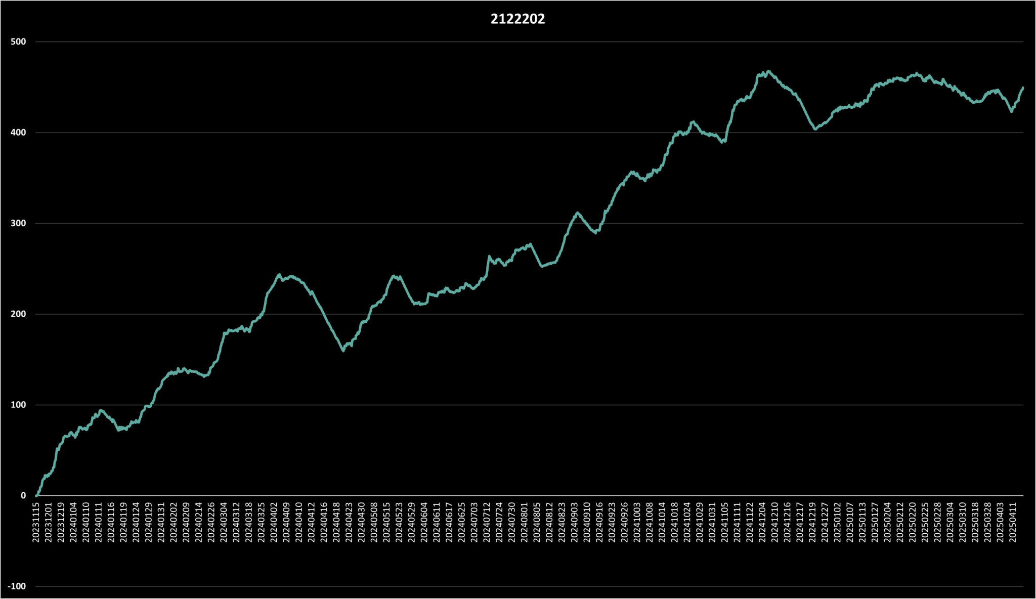
Figure 5.2.b — Return per Time Curve for System 2122202
This chart illustrates the Return per Time performance of System 2122202, tested across 200 tickers between 2023 and 2025. Unlike many strategies that plateau or reverse during the final year, this system sustains an upward-sloping equity curve—showcasing durability and adaptability. Its resilience throughout shifting market conditions makes it a standout candidate for further development.
| Return | RpT | Trades |
2023 | 65.55 | 0.8311 | 79 |
2024 | 359.61 | 0.2025 | 1776 |
2025 | 24.1 | 0.0557 | 433 |
Table 5.2.b — Annual Breakdown for System 2122202
This table summarizes the year-by-year performance for System 2122202. Despite natural softening in per-trade profitability as the system scales up, returns remain positive throughout the test period. The trade count is healthy, and even in 2025—the year where most systems deteriorated—the model continues to generate profits.
6. Next Steps: Final Fine-Tuning
Now that System 2122202 has demonstrated consistency across time, solid return characteristics, and a reasonable trade volume, I believe it’s ready for a refinement phase. The objective at this point is not to force better results, but to sharpen the system’s focus—isolating the higher-quality trade setups while avoiding unnecessary complexity.
While this configuration already uses six distinct indicators, and I generally favor minimalist rule sets for the sake of generalization and operational simplicity, I’m open to introducing a seventh condition—if it improves precision or improves the system’s risk/reward posture while reducing the quantity of trades to a manageable level. In other words, any addition must earn its place by enhancing system behavior without degrading interpretability or manageability.
That said, there’s always the tempting alternative: tweaking the numeric parameters of the existing triggers to optimize performance. But that’s a dangerous path—one that often leads to overfitting. When you tailor a system too closely to historical data, it tends to perform well only within that sample—failing to generalize to live market conditions where the variables are far less cooperative.
Instead of optimizing the past, my focus is on building a system that remains structurally robust across changing environments. That means evaluating performance not just by metrics like return or win rate, but by examining behavior across different regimes, timeframes, and tickers.
The goal here isn’t perfection—it’s durability. I’m not trying to engineer the highest-returning system on paper. I’m trying to build something I can trust, trade, and scale with discipline. By continuing to let the data lead—and resisting the urge to force-fit results—I aim to construct a system that not only performs in backtests but hopefully also holds up in the future data.
6.1 Exploring Trade Adjustments with New Conditions
To further enhance the trade quality within System 2122202, I introduced a new entry filter: requiring that the close be below EMA[C, 50] minus ATR[TR, 13] at the time of entry. The aim here isn’t to over-optimize, but rather to eliminate setups where price remains relatively elevated—often signaling that a pullback hasn’t yet matured or that downside risk still outweighs upside potential.
This isn’t about tightening the rules just to see metrics improve. It’s about improving the risk-reward quality of the signals by excluding trades that—historically—have underperformed or contributed to drawdowns.
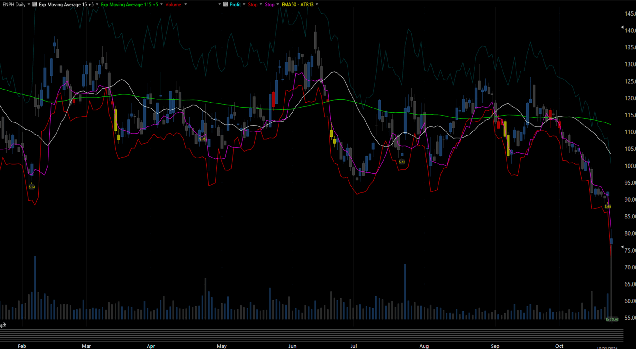
Figure 6.1.a — Visualizing the New Entry Filter
This chart shows how the new condition (C < EMA[C, 50] – ATR[TR, 13]) impacts system behavior for ENPH from January to October 2024. The white line marks the dynamic threshold set by this condition. Trades that would have triggered above this line are now excluded (marked red candles)—many of which previously led to poor outcomes. Notice how this adjustment successfully filtered out several weak entries, including those from early and late September 2024.
What’s particularly satisfying is how this new rule stepped in and did its job cleanly on the first try—like a supporting actor nailing their part without hijacking the plot. It added meaningful selectivity without drastically reducing the system’s ability to participate in profitable trades.
Best of all, it accomplished this without parameter over-tweaking or logic overload. Just one clean rule, plugged in with intent—and it worked. This is the kind of rare moment in system design that feels like hitting a 280-yard drive during warm-up, coffee still in hand.
Here’s a quick side-by-side of the system’s behavior with and without this filter applied:
|
Metric |
With Condition |
Without Condition |
|
Trades |
445 |
2288 |
|
Binary |
2122202 |
|
|
Return |
133.53 |
449.37 |
|
RpT |
0.3001 |
0.1964 |
|
B.A |
60.67 |
57.94 |
|
Avg Holding Time |
9.0 days |
8.2 days |
Table 6.1.a — Parameter Comparison With vs. Without the New Filter
This table highlights the trade-off introduced by the filter: fewer trades and lower total return, but with significantly improved Return per Trade and Batting Average. This means fewer, but better trades—an ideal refinement in swing systems where risk control and trade efficiency are often more valuable than sheer trade volume.
The Bigger Picture
Removing 80% of the trades will obviously reduce the total return—that’s not surprising. What is meaningful is how the trades that remain are higher quality, with improved consistency and risk-adjusted outcomes.
This kind of evolution—where trade count goes down but trade clarity and payoff go up—is exactly the kind of shift that makes systems more durable in live conditions. Lower noise, lower stress, and higher confidence in the logic driving each entry.
So, where do we go from here?
This seems like the perfect time to expand testing across other tickers. If the same uplift holds, we may have uncovered a scalable adjustment that tightens the edge. If not, the results themselves will guide the next iteration—just as they should.
6.1.1. Enhanced Performance with Targeted Entry Filter
Following the promising results of System 2122202, I introduced a new condition—C < EMA[C, 50] – ATR[TR, 13]—designed to eliminate trades occurring when price remains relatively elevated above a dynamic trend-volatility threshold. The intent was to exclude weaker setups that historically led to poor outcomes while maintaining enough trade activity for the system to remain operationally useful.
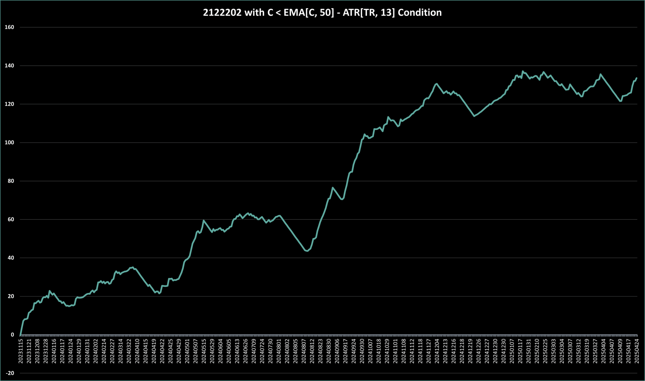
Figure 6.1.b — Enhanced Equity Curve for System 2122202
This chart visualizes the performance of System 2122202 across approximately 200 U.S. equity tickers over a two-year period (March 2023 to April 2025), following the addition of the entry filter C < EMA[C, 50] – ATR[TR, 13]. The updated system exhibits smoother equity growth, reduced volatility, and fewer sharp drawdowns—highlighting the filter’s ability to exclude weaker setups while preserving upside potential. The result is a more disciplined and resilient strategy profile, particularly valuable in uncertain or choppy market environments.
“– ATR[TR, 13]” —designed to eliminate trades occurring when price remains relatively elevated above a dynamic trend-volatility threshold. The intent was to exclude weaker setups that historically led to poor outcomes while maintaining enough trade activity for the system to remain operationally useful.
6.1.2. A Year-by-Year Breakdown
To quantify the effect of the new condition, I analyzed the strategy’s performance across three calendar years. The table below breaks down total return, return per trade (RpT), and number of trades per year.
| Return | RpT | Trades |
2023 | 19.5 | 1.03 | 19 |
2024 | 105.83 | 0.32 | 331 |
2025 | 8.2 | 0.09 | 95 |
Table 6.1.b — Yearly breakdown of System 2122202 with C < EMA[C, 50] – ATR[TR, 13] condition applied.
6.1.3 Interpretation
This year-by-year breakdown reinforces the effectiveness of the newly added filter: C < EMA[C, 50] – ATR[TR, 13]. Return, RpT and the number of trades all changed less comparing to the unfiltered version, especially in 2023 and 2024. Even in 2025—a year where many strategies experienced performance decay—the refined system maintained positive returns and held a respectable RpT.
What’s especially encouraging is how this filter boosts statistical discipline without introducing unnecessary rigidity. It filters out trades that occur too early in retracements or too close to short-term tops—common culprits for whipsaws and stop-outs.
This supports one of my core design principles:
“A better system isn’t built on more complexity—it’s built on better timing.“
Instead of chasing returns by over-optimizing, a well-placed filter can meaningfully shift trade quality by aligning entries with more favorable price locations. In this case, the added condition enhances risk control without gutting opportunity or overwhelming the system with logic layers.
6.1.4 Refinement Through Parameter Exploration: EMA Period Optimization
While 2024 was strong for the refined system, performance in 2025 showed a softening trend—particularly in RpT and batting average, even as trade frequency remained stable. This hinted at an opportunity to revisit and experiment with the newly added filter, specifically the EMA period used in the condition.
The original formulation used EMA[C, 50], but adjusting this parameter could improve the system’s adaptability across different market conditions. Instead of choosing values arbitrarily, I opted to test Fibonacci-based EMA periods, which offer a natural progression of sensitivity levels common in technical analysis.
Here’s a breakdown of the tested values:
- EMA[13] – Very responsive to short-term movement. Ideal for fast-trading systems, but prone to noise.
- EMA[21] – A smoother short-term filter, offering a better balance between reactivity and noise control.
- EMA[34] – A mid-range tracker, often used to capture consistent trend behavior.
- EMA[50] – The baseline filter previously used. Sits in the sweet spot of short- and medium-term smoothing.
- EMA[55] – Slightly slower than 50, capturing deeper retracements and more structured trends.
- EMA[89] – A long-term filter. Reduces reactivity but can confirm larger directional movements.
The revised filter condition tested across each period was:
C < EMA[C, (Eny of the above)] – ATR[TR, 13]
The purpose of this experiment isn’t to find a perfect-fit parameter for historical data—it’s to observe how trend sensitivity impacts signal quality and to discover which EMA periods offer the best blend of profitability, stability, and selectivity across the system’s architecture.
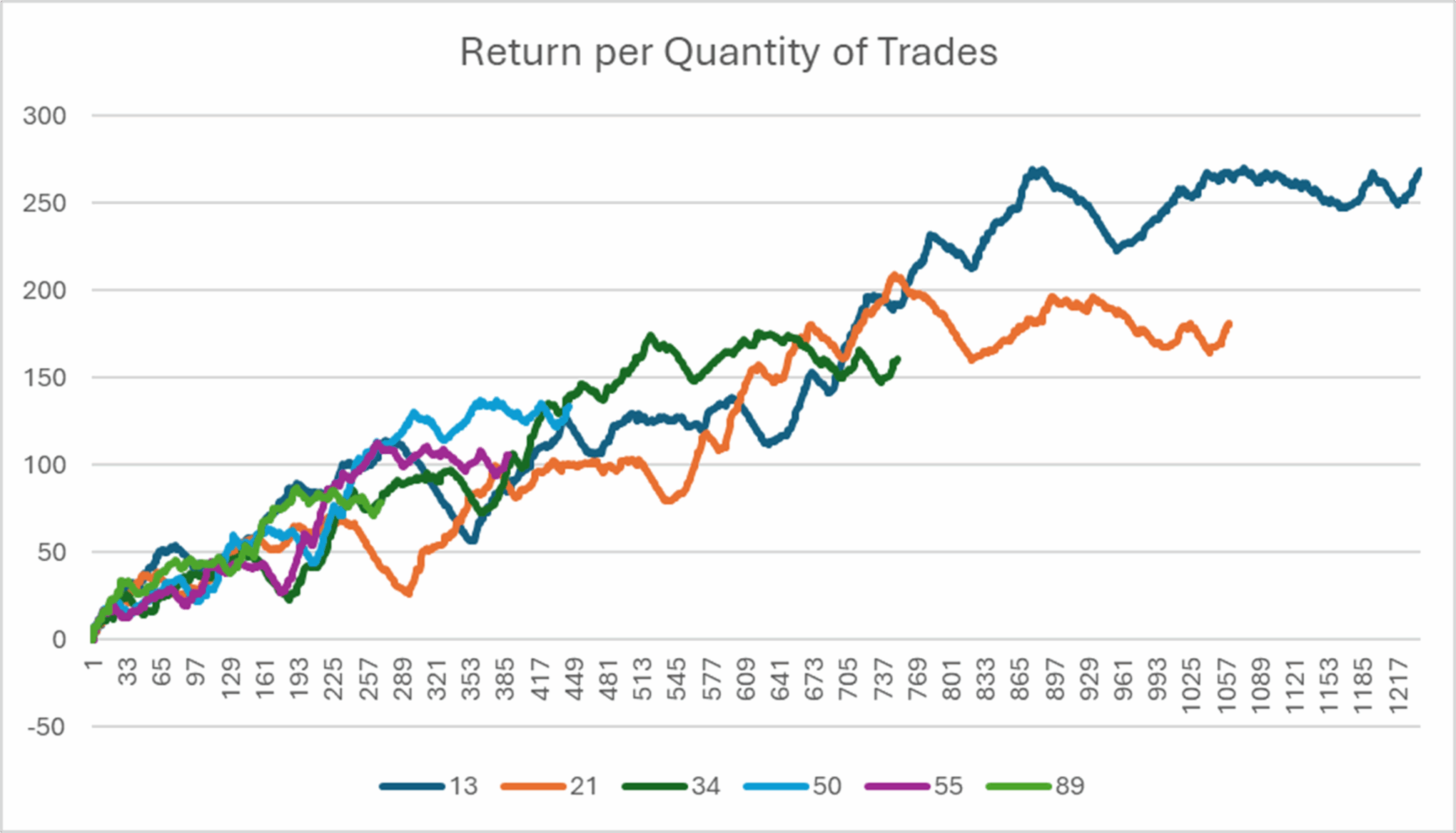
Figure 6.1.c — Return per Quantity of Trades by EMA Filter
This chart visualizes cumulative return as a function of trade quantity for System 1220102, using six different EMA periods (13, 21, 34, 50, 55, 89) within the refined entry condition:
C < EMA[C, (Eny of the above)] – ATR[TR, 13]
The chart clearly highlights how EMA[50] consistently outperforms other variants, offering a rare balance of return stability and trade frequency. Systems using shorter EMAs (13, 21) tend to burn out faster, while longer EMAs like 89 are too selective, failing to compound over time.
This visual supports the decision to stick with EMA[50] as the anchor point. It demonstrates that optimal signal quality often lies not at the extremes, but in the middle—where enough trades occur to create reliability, yet the filter is strong enough to eliminate noise.
6.2 Finding the Sweet Spot: Is This the System’s Natural Ceiling?
When looking at the chart, it’s easy to be drawn to the variation that posts the highest return. Especially when performance patterns across the different EMA values appear similar, the temptation is to default to the most profitable version. But that prompts a critical question:
Why accept fewer trades unless those trades are demonstrably better?
That’s the trade-off this analysis was designed to explore. Longer EMA values often succeed in filtering out noise—but they do so at the cost of reduced trade volume. The key is finding the point where trade quality improves without bleeding too much opportunity.
The results are both surprising and encouraging. Of all the tested configurations, the original filter—C < EMA[C, 50] – ATR[TR, 13]—emerged as the optimal balance. It preserved a practical number of trades while also producing the highest Return per Trade (RpT) and total return. That’s a rare and valuable outcome—since, in system development, gains in precision often come with a steep price in trade frequency.
Even more telling: the batting average for EMA[50] also outperformed most other configurations. This reinforces that the filter doesn’t just cut out bad trades—it consistently keeps the ones worth holding. The EMA[50] setting isn’t just “good enough.” It appears to be a genuine sweet spot—responsive enough to catch meaningful setups, but stable enough to sidestep the whiplash of short-term noise.
But with that clarity comes a new question:
Have we reached this system’s natural ceiling?
Or can we still improve by experimenting with:
- Different ATR multipliers
- Smarter, adaptive filters based on volatility or regime changes
- Refinements to exit logic, designed to match different types of entries
That’s the path forward. But for now, we’ve uncovered a configuration that offers rare consistency—a strong, balanced foundation worth refining further.
6.2.1 Comparing EMA Periods:
EMA Period | Trades | Total Return | RpT | Batting Average (B.A) |
13 | 1239 | 268.67 | 0.22 | 56.06 |
21 | 1061 | 181.37 | 0.17 | 54.62 |
34 | 751 | 160.83 | 0.21 | 57.52 |
50 | 445 | 133.53 | 0.3 | 60.67 |
55 | 389 | 105.96 | 0.27 | 59.9 |
89 | 270 | 78.75 | 0.29 | 61.85 |
Table 6.2.a — System 2122202 with C < EMA[C, (Any of the above] – ATR[TR, 13] Condition Applied
The EMA[50] filter stands out by achieving the highest total return and RpT, with a batting average second only to EMA[89]—but at significantly slower trade frequency, resulting with smaller return.
6.2.2 Refining Precision: Testing the Impact of ATR Multiplier Adjustments
After establishing a strong foundation with the C < EMA[C, 50] – ATR[TR, 13] condition, it’s only natural to ask: Can we make it better?
This filter already delivers the highest Return per Trade (RpT) among all tested variants, maintains a reasonable trade volume, and ranks second in Batting Average (B.A.). It’s a rare intersection of quality and consistency—two traits every systematic trader aims to preserve.
But what if the EMA[50] threshold could be fine-tuned with a more dynamic volatility buffer?
To answer that, I ran a focused test adjusting the ATR multiplier in the filter condition.
Tested Variants:
Each version applies a different multiplier to the ATR component of the condition:
- +2 ATR — A loose filter allowing early entries; often aggressive and riskier.
- +1 ATR — Moderately aggressive; admits trades earlier in a swing.
- 0 ATR — Pure EMA filter, removes volatility adjustment entirely.
- -1 ATR — The original configuration; a balanced, conservative filter.
- -2 ATR — Ultra-selective; potentially too restrictive for active trading.
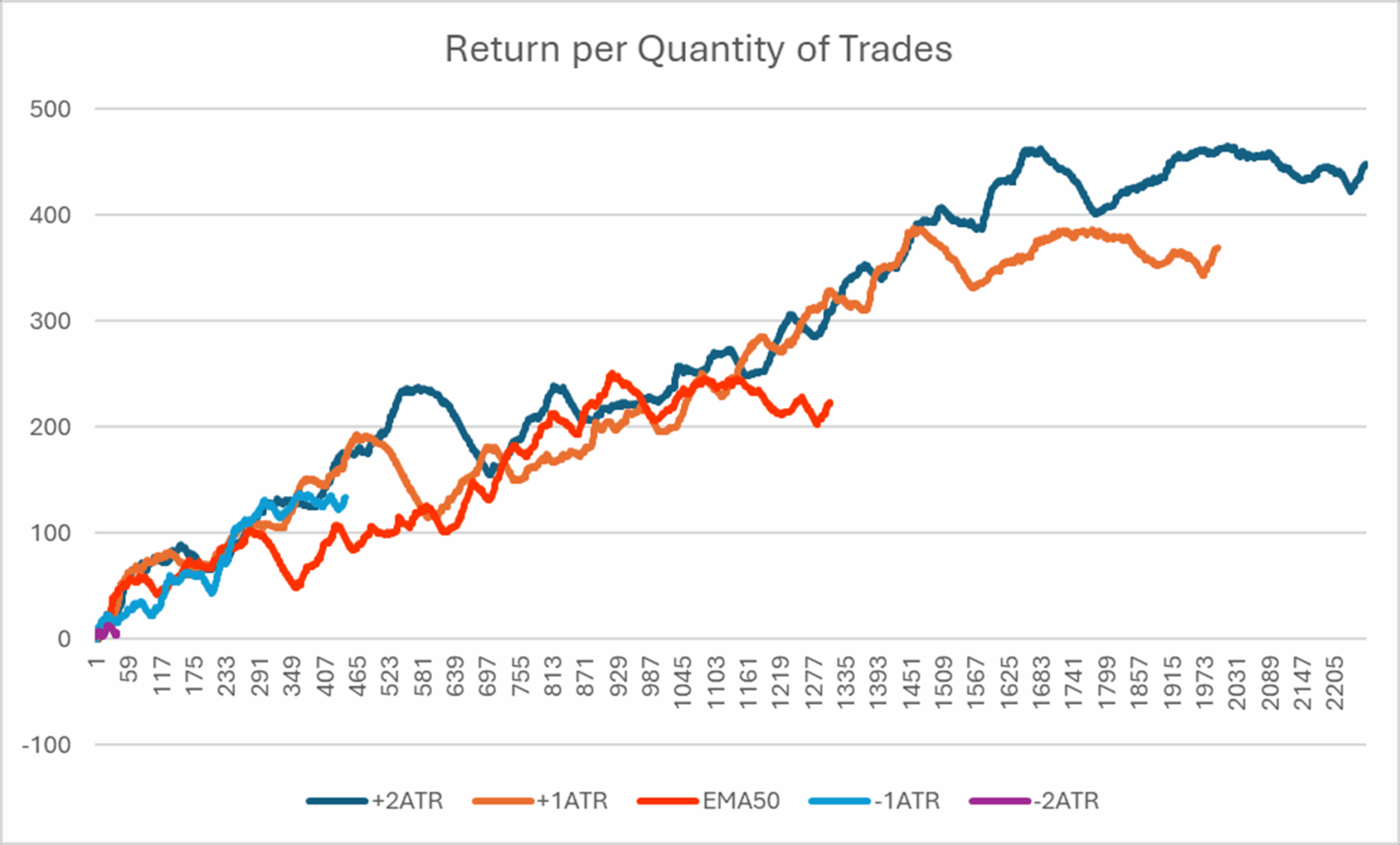
Figure 6.2.a — ATR Multiplier vs. Return per Trade
This chart tracks the cumulative return of System 2122202 under five different ATR multiplier settings. It shows how varying the volatility buffer influences trade behavior and profitability. Systems with tighter filters (like -1 or -2 ATR) tend to exhibit higher RpT but fewer trades, while more permissive filters (+1 and +2 ATR) increase participation but dilute trade quality.
ATR Multiplier | Trades | Total Return | RpT | Batting Average (B.A.) |
2 | 2,262 | 449 | 0.20 | 0.56 |
1 | 1,998 | 370 | 0.19 | 0.55 |
0 | 1,308 | 223 | 0.17 | 0.58 |
–1 | 445 | 134 | 0.30 | 0.61 |
–2 | 39 | 6 | 0.15 | 0.60 |
Table 6.2.b — System 2122202 with ATR Variations Applied
Key Takeaways
- -1 ATR remains the sweet spot: It delivers the best RpT and highest win rate, confirming its effectiveness in filtering trades that are both well-positioned and well-timed.
- Aggressive entries (+1, +2 ATR) bring more trades, but performance becomes increasingly inconsistent.
- Over-tightening (-2 ATR) leads to under-trading: too few setups, and the system becomes statistically fragile.
This analysis confirms the power of small parameter shifts. The optimal system wasn’t improved by brute-force optimization or additional layers—it simply emerged as the best fit from the beginning.
Next, I’ll explore the impact of tuning exit rules in a similarly methodical way. Because once entries are solid, the exit is where performance is either crystallized—or squandered.
7. Final Thoughts: Why I’m Sticking With the Original
At first glance, the more aggressive filter variations—such as +1ATR or +2ATR in the entry condition—may seem appealing. Their equity curves boast higher cumulative returns, and the prospect of capturing trades earlier in the cycle is tempting. But a deeper analysis reveals a more grounded reality.
Shifting away from the original –1ATR filter consistently reduced the system’s Return per Trade (RpT) and introduced greater instability. These variants often achieved their results at the cost of trade quality, highlighting an essential trade-off between selectivity and noise. The illusion of improvement is a common pitfall in system optimization: tweaking parameters until the backtest looks impressive, only to discover that the logic crumbles in real-world conditions.
This is why I’m anchoring my strategy to the original setting: Close < EMA[50] – ATR[13]. It may not deliver the flashiest curve, but it consistently filters out high-risk trades and positions entries closer to structurally favorable price zones. This stability is far more valuable than chasing slightly higher theoretical returns with increased risk.
Wrapping Up This Phase
This phase of the project isn’t about claiming to have found “the best” trading system. It’s about demonstrating a research-driven process for refining system logic—and importantly, resisting the urge to over-optimize. Every iteration was grounded in data, and each modification tested against the realities of changing market conditions.
For now, I’m saving this version of System 2122202 with the –1ATR entry filter. It will enter a forward-testing phase where I’ll observe its real-time behavior. If it continues to perform reliably, I may begin limited live deployment using conservative sizing (e.g., 1% risk per trade).
A key strength of this system is its long-only structure, tailored to capture upward momentum during favorable setups. And the addition of this new filter—excluding trades where the close remains elevated above the EMA-based threshold—has significantly enhanced its entry logic. By focusing on areas of relative weakness (local lows), the system improves its edge while avoiding overexposure near short-term highs.
Visualizing the Filter in Action
To illustrate the practical impact of this filter, I’ve included two annotated charts below.
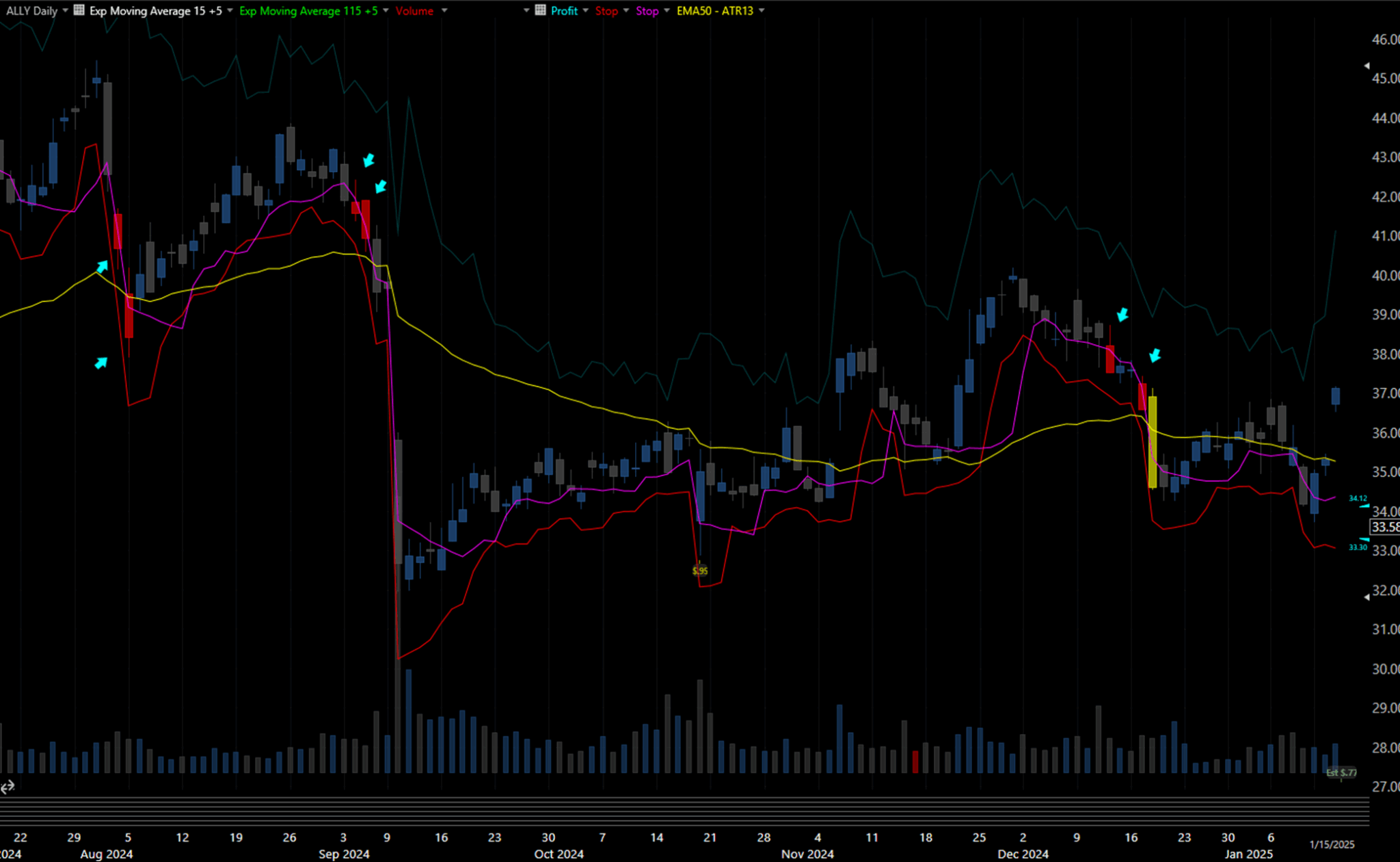
Figure 7.a — Filtered Trade Positioning (ALLY, Jul–Dec 2024)
This chart shows how the updated entry condition filters out weak setups. Notice that trades previously clustered near local highs are now excluded (Cyen Arrow). The yellow threshold line (EMA[50] – ATR[13]) visually marks the new trade barrier. Only those candles that close below it are now considered for entry. Notably, the remaining trades tend to appear closer to local price troughs, such as in early August, September, and December—offering improved entry timing and better potential for follow-through.
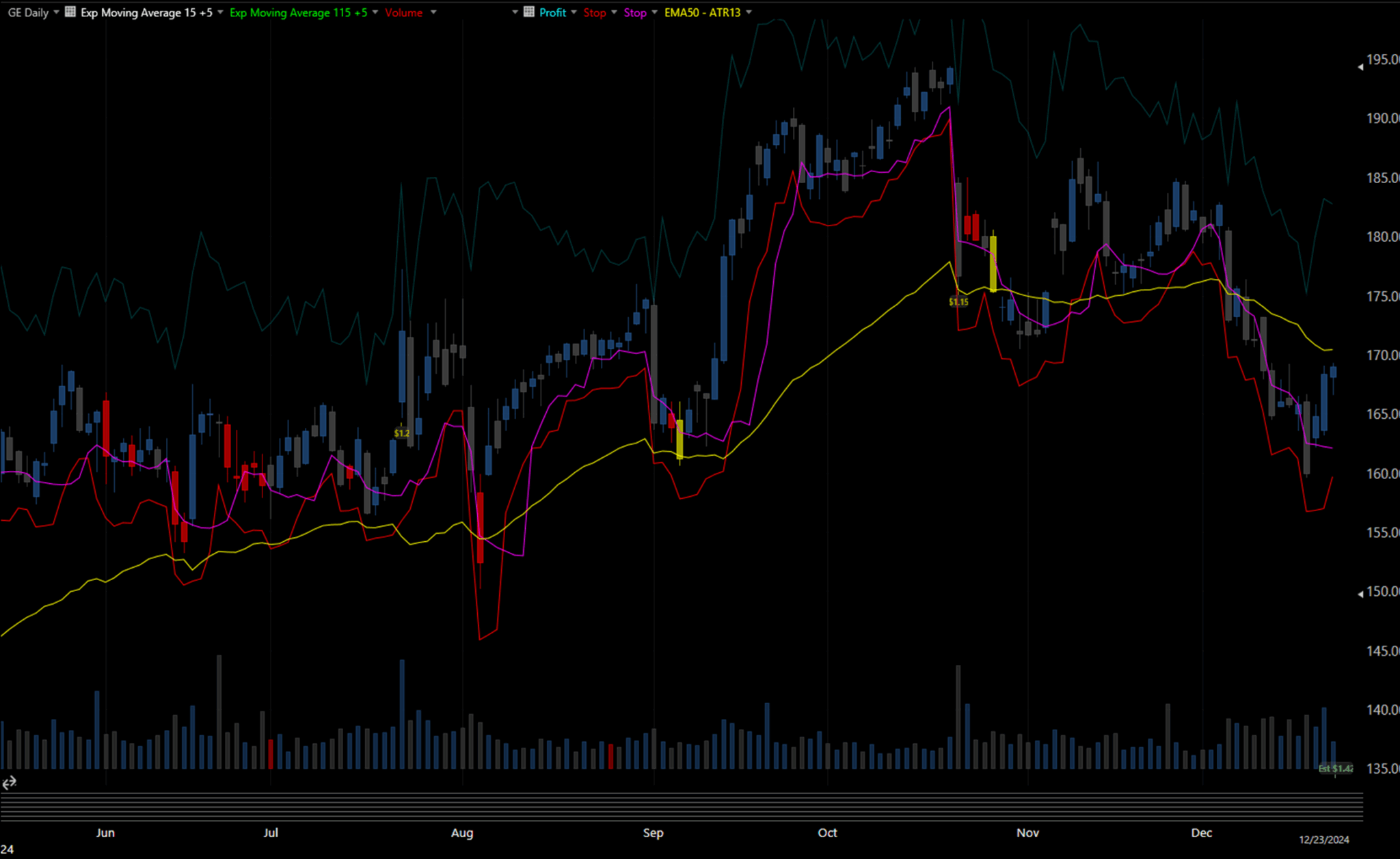
Figure 7.b — Enhanced Entry Filtering on GE (May 2024 – Jan 2025)
In this GE chart, the same filter is applied, and again the results are telling. Trades previously triggered near short-term price spikes are now eliminated. The system becomes more selective without sacrificing structure or clarity. Over 80% of weak or late entries are filtered out, leaving behind a core set of higher-quality opportunities.
This reinforces the broader insight: a well-placed filter can do more than cut risk—it can elevate the entire system. The updated 2122202 strategy does exactly that, not by adding complexity, but by aligning trades with structurally sound market behavior.
This isn’t the end of the journey. But it is a solid milestone—a filtered, tested, and logically sound foundation that I can now build on with confidence.
7.1 Final System Results: Performance Snapshot
After all refinements and iterations, the system reaches a well-rounded performance profile that balances trade quality, frequency, and risk control. Below are the final performance metrics:
Metric | Value |
Total Trades | 445 |
Total Return | 133.53% |
Return per Trade (RpT) | 0.3001% |
Batting Average (Win Rate) | 60.67% |
Average Holding Time (All Trades) | 9.0 days |
A.H.T. – Winning Trades | 11.1 days |
A.H.T. – Losing Trades | 5.7 days |
A.H.T. to Hit Profit Target | 13.2 days |
A.H.T. to Hit Stop Loss | 4.9 days |
A.H.T. to Hit Trailing Stop | 10.7 days |
Total Value Gained | +284.00% |
Total Value Lost | –150.48% |
Winning Trades | 270 |
Losing Trades | 175 |
Max Return (Single Trade) | 3.84% |
Max Loss (Single Trade) | –1.03% |
Average Return (Winners) | 1.05% |
Average Loss (Losers) | –0.86% |
What stands out most is the system’s consistency: a healthy win rate above 60%, a respectable RpT near 0.30%, and clear evidence of effective exit logic—seen in the faster resolution of losing trades and extended holding of profitable ones. This mix of discipline and edge is what gives the strategy real-world potential.
7.2 Trade Examples: From Theory to Execution
Backtest statistics give us the big picture, but trade-by-trade examples breathe life into the data. These annotated chart snapshots show how the system performed in the wild—where entries occurred, how profits were captured, and when the stops protected capital.
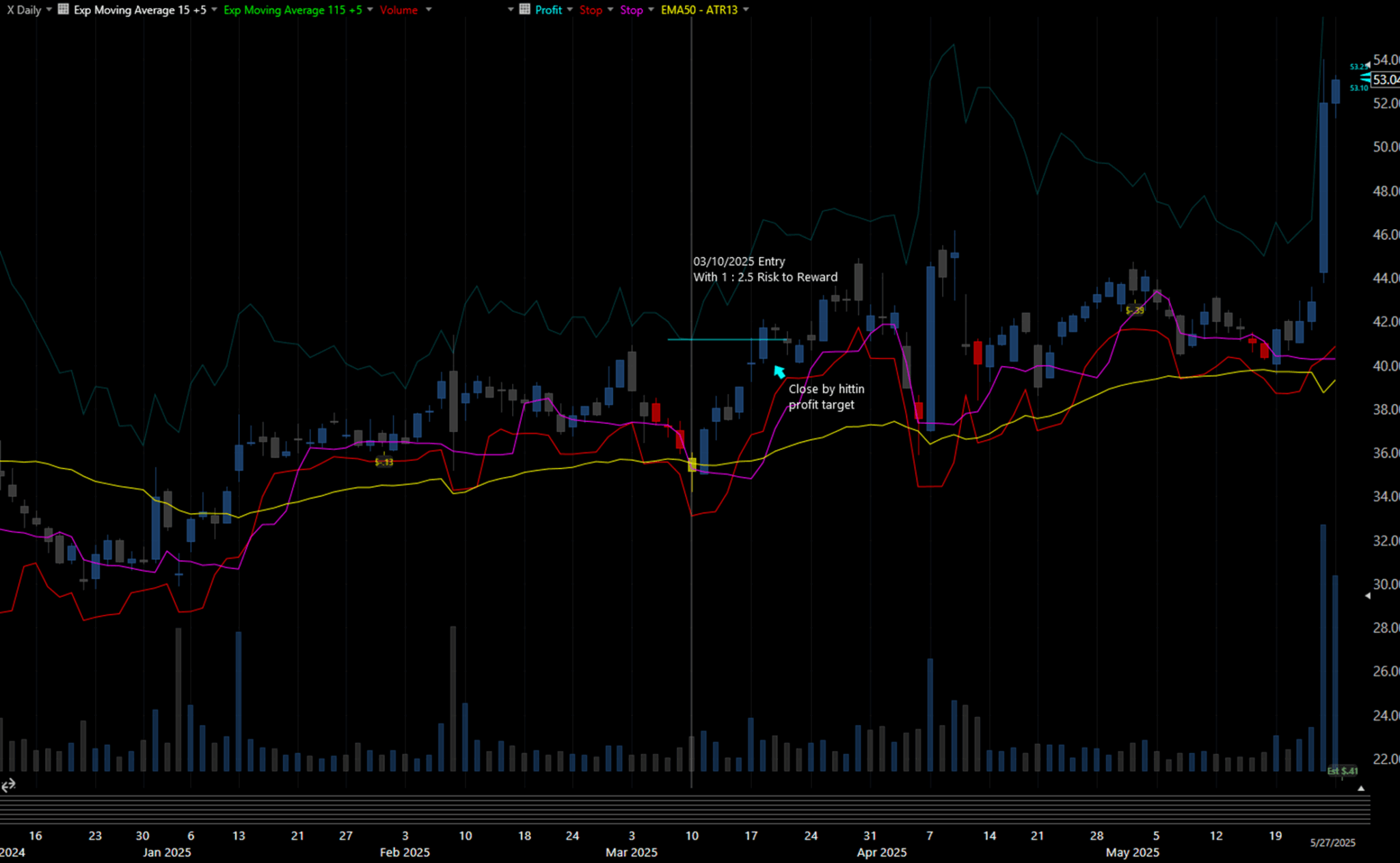
Figure 7.2.a — System Entry on X (Jan–May 2025)
This trade exemplifies textbook execution: the system enters on a signal that aligns with the refined filter and exits by hitting the 2.5x risk reward target. The entry came just after a minor pullback, catching the move near the base and riding it with precision to the exit.
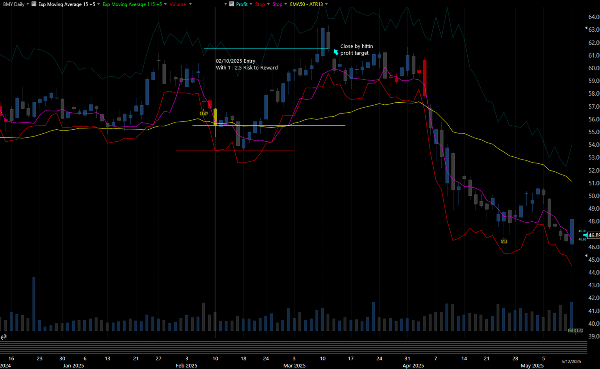
Figure 7.2.b — Trade on BMY (Dec 2024 – May 2025)
Here we see a perfect example of persistence paying off. Although the position hovered near the stop-loss zone just a few days after entry, it survived and rallied directly to the profit target. The trailing stop nearly closed the trade early, but the system’s rules held, resulting in a clean win.
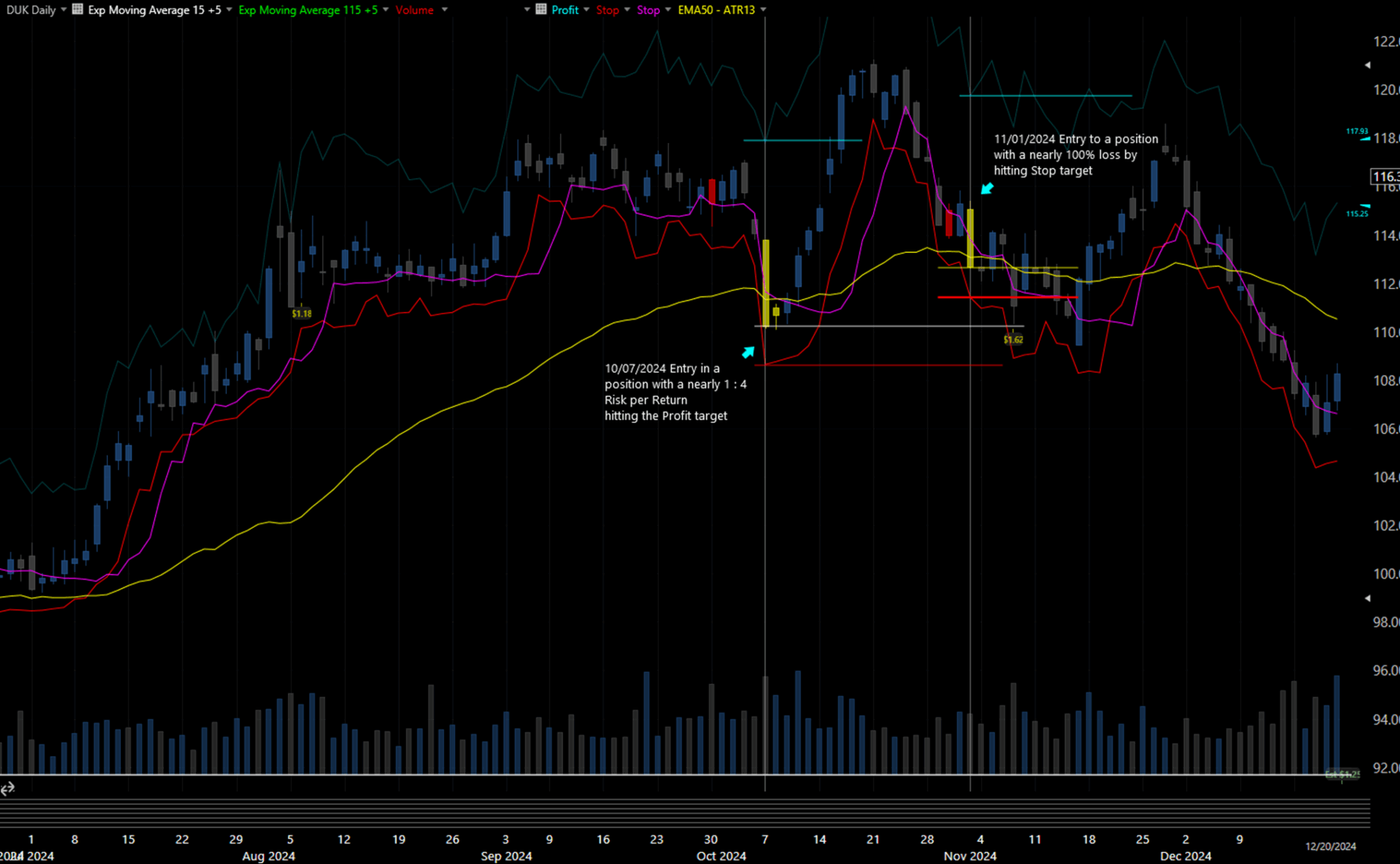
Figure 7.2.c — Mixed Outcomes on DUK (Jul–Dec 2024)
To keep things honest, this final chart shows two back-to-back trades: one winning, one losing. The first yielded nearly 4x risk before closing on target. The second, entered just weeks later, hit its stop for a full loss. This side-by-side contrast reminds us that even the best systems come with setbacks—but the net edge lies in risk management and reward asymmetry.
Wrapping Up – And This Is Just the Beginning
Thanks for reading this deep dive into the development and refinement of a long-only, rule-based trading system. This project reflects hundreds of hours of testing, tuning, and validating ideas—not just to chase returns, but to create something consistent, explainable, and scalable.
🔍 What’s Next?
- I’ll continue testing live results and adapting based on new data.
- Expect future posts exploring system variations, broader market filters, and multi-regime logic.
- And yes—short-side testing is coming.
Support, Customization, and Collaboration
If this kind of system design interests you, there are a few ways you can engage further:
 Feedback — Leave a comment with questions, critiques, or suggestions. I read everything.
 Custom Strategy Tuning — I offer personalized logic adjustment or tailored testing (fee-based). If you have a trading idea you want evaluated in this framework, feel free to reach out.
 Subscribe — If you found value in this work, subscribing to the paid tier supports more content like this—and gives you early access to future tools and research.
This is just the beginning of a larger library I’m building around practical, data-backed trading systems. Thank you again for being part of the journey.
More soon.
— End of Part One
⚠️ Disclaimer
The content provided in this post is for informational and educational purposes only. It represents my personal research, observations, and experimentation with trading systems, and is not intended as financial advice, investment advice, or a recommendation to buy or sell any securities or financial instruments.
Trading in the financial markets involves significant risk, and you should never invest money you cannot afford to lose. The systems discussed here were tested using historical data under specific assumptions, and past performance is not indicative of future results. Market conditions change, and no strategy can guarantee profits or prevent losses.
While I strive to be as transparent and data-driven as possible, all results, charts, and conclusions are presented as-is and may contain errors, omissions, or inaccuracies. Any decisions to trade based on this content are made entirely at your own risk. I disclaim all liability for any financial loss, damage, or consequences that may result from the use of the information provided here.
Please consult with a licensed financial advisor, legal professional, or risk specialist before engaging in any trading or investment activity.